


What Is Sentence Embedding?
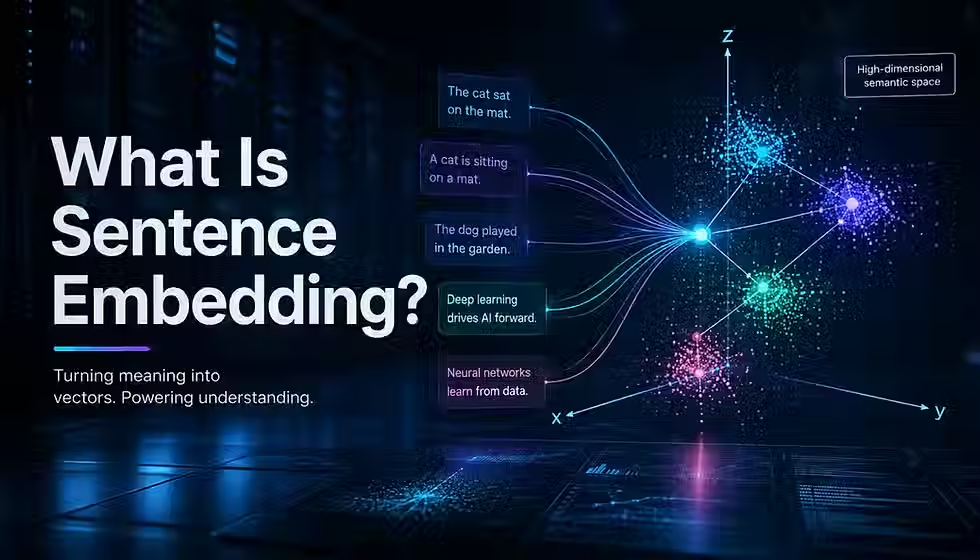
Type "my card was declined twice" into a search box, and a good support system should also surface an article titled "why did my payment fail." No word is shared between those two phrases, yet they mean nearly the same thing. A computer matching only letters misses that connection entirely. A computer that has learned to represent meaning as numbers does not. That capability — turning sentences into numbers that capture what they mean rather than which words they use — is what sentence embedding does, and it quietly powers everything from support search to the retrieval step inside modern AI assistants.
TL;DR
A sentence embedding is a fixed-length numerical vector representing a sentence's meaning, so similar sentences land close together in vector space.
Most modern sentence embeddings come from transformer models: text is tokenized, passed through transformer layers, pooled into one vector, and often normalized.
Similarity is usually measured with cosine similarity or a dot product — not a single universal "same meaning" threshold.
Sentence embeddings power semantic search, retrieval-augmented generation (RAG), clustering, deduplication, classification, and recommendations.
No model is best at everything; choice depends on task, domain, language, latency, and cost, validated on your own data.
Embeddings capture topical similarity well but can be fooled by negation, numbers, and fine-grained facts, so high-stakes systems still need reranking or verification.
What Is Sentence Embedding?
A sentence embedding is a fixed-length numerical vector produced by a machine learning model that represents a sentence's meaning. Sentences with similar meaning sit near each other in this vector space, while unrelated sentences sit farther apart. Sentence embeddings power semantic search, letting a system match a query to relevant text by meaning instead of exact keywords.
Table of Contents
What Sentence Embedding Actually Means
In machine learning, an "embedding" is a learned mapping from a piece of data — a word, image, product, or sentence — to a point in a numerical vector space. A vector is simply an ordered list of numbers. A sentence embedding applies that idea to a full sentence: a model reads it and outputs a fixed-length list of numbers, typically 256 to 4,096 values, standing in for its meaning.
The organizing principle is distance. Sentences the model judges as similar sit close together; unrelated sentences sit farther apart. This differs from a hash or ID, where near-identical inputs can land anywhere. It also differs from a database record: an embedding doesn't store the sentence's text, and you cannot decode the original words back out. It is a compressed, distributed representation — not a summary, not a lossless encoding.
Consider three sentences: (1) "The flight was delayed because of bad weather." (2) "Bad weather pushed the departure time back." (3) "The chef added too much salt to the soup." Sentences 1 and 2 describe the same event with different words, so a well-trained model should place their vectors close together. Sentence 3 is unrelated and should sit much farther away. Nobody can state exact coordinates without running a real model, and this guide won't invent numbers that look official but aren't — what matters is the pattern: near-duplicate meaning produces near-duplicate vectors.
"Sentence embedding" is used loosely in practice, covering short phrases, queries, and even paragraph-length passages. Practitioners rarely draw a hard line between "sentence" and "passage" encoders — it's more about training data and typical input length than a fixed rule within machine learning.
It's also worth being precise about what an embedding is not. It doesn't store exact wording or facts, and no single dimension corresponds to a clean, nameable concept like "topic: sports." The feature space a transformer learns is distributed: meaning spreads across many dimensions working together, not localized to one.
Sentence Embeddings vs. Related Representations
Several neighboring terms get conflated, and mixing them up leads to real engineering mistakes.
Word embeddings map individual words to vectors independent of context — "bank" gets one vector whether it means riverbank or savings bank. Token embeddings are the raw input vectors a transformer looks up per subword token, also context-free. Contextual token representations are a transformer's internal-layer outputs — now "bank" differs by sentence, since self-attention lets every token absorb surrounding context. A sentence embedding condenses an entire sequence of these into one fixed-length vector via pooling.
Document or passage embeddings apply the same idea to longer spans; the sentence/passage boundary is practical, not strict.
One-hot vectors are sparse and arbitrary — each category gets its own dimension with no learned notion of similarity, as covered in this guide to one-hot encoding. Dense sentence embeddings solve exactly what one-hot vectors can't: placing related meanings near each other.
That sparse-vs-dense split shows up in retrieval too. Sparse retrieval (TF-IDF, BM25) scores documents by shared, weighted words — fast and exact-match-friendly but blind to paraphrase. Dense retrieval uses embeddings and matches "physician" to "doctor" with no shared characters, but can miss rare exact terms like a product SKU. Many production systems combine both as hybrid search.
Semantic search describes finding results by meaning; keyword search by literal terms. Bi-encoders embed each text independently so document vectors can be precomputed and reused; cross-encoders score a pair jointly, more accurate but not precomputable. Finally, embedding models output vectors representing meaning, while generative language models produce new text — RAG systems typically use both together.
Concept | Represents | Precomputable? | Typical use |
Word embedding | Single word, context-free | Yes | Legacy NLP |
Contextual token representation | Token, context-aware | No | Intermediate transformer state |
Sentence embedding | Sentence/short passage | Yes | Semantic search, clustering, RAG |
One-hot vector | Category identity | Yes | Categorical features |
Sparse retrieval score | Term overlap | Partially | Exact keyword matching |
Why Sentence Embeddings Matter
Keyword matching fails predictably: it cannot handle synonyms, paraphrase, or differently worded questions sharing the same intent. Lexical mismatch is one of the oldest unsolved problems in retrieval, and it's exactly what dense embeddings target.
There's also an efficiency argument. Comparing every possible text pair directly, as a cross-encoder would, doesn't scale. Reimers and Gurevych's Sentence-BERT paper reported finding the most similar pair among 10,000 sentences took roughly 65 hours with raw BERT cross-encoding, versus about 5 seconds once sentences were embedded and compared with cosine similarity, because each embedding only needs computing once and can be reused for any number of comparisons [1]. That gap — precompute once, compare cheaply and repeatedly — is why embeddings, not pairwise scoring, underpin large-scale search.
Sentence embeddings also enable transfer learning: one pretrained encoder's vectors can feed classification, clustering, and retrieval without retraining a new model for each task.
A Short History of Sentence Representations
Sparse, frequency-based methods came first — bag-of-words, TF-IDF, BM25 — representing text purely by which words appeared, with no notion of meaning beyond overlap.
Distributed word embeddings changed that. Word2vec (Mikolov et al., Google, 2013) learned dense word vectors by predicting context, producing vectors where related words landed near each other [2]. GloVe (Pennington, Socher, and Manning, Stanford, 2014) derived word vectors from corpus-wide co-occurrence statistics [3]. Both were breakthroughs for word-level meaning but didn't specify how to represent a whole sentence.
Averaging word vectors into one sentence vector was the direct early answer — simple and fast, but it loses word order and negation: "the dog bit the man" and "the man bit the dog" can average to nearly identical vectors despite opposite meanings.
Supervised recurrent and convolutional encoders followed, training networks explicitly for sentence vectors using labeled data like natural language inference pairs (InferSent being an influential example).
Contextual transformer representations changed the underlying machinery: every token's representation now depends on the whole surrounding sentence via stacked self-attention.
BERT (Devlin et al., Google, 2019) became the dominant pretrained transformer encoder, but its native [CLS] output wasn't designed as a general-purpose sentence embedding — raw BERT [CLS] vectors perform poorly on similarity tasks, since BERT's pretraining objectives don't directly optimize for placing similar sentences near each other [1].
Universal Sentence Encoder (Cer et al., Google, 2018) offered an early widely used general-purpose encoder, in both transformer and lighter Deep Averaging Network variants, trained explicitly for transfer to many tasks [4].
Sentence-BERT (Reimers and Gurevych, 2019) fixed the "raw BERT is a poor sentence encoder" problem directly, fine-tuning BERT with a siamese network so pooled output can be compared with cosine similarity [1], becoming the foundation of the widely used Sentence Transformers library.
Contrastive and instruction-aware models came next. SimCSE (Gao, Yao, and Chen, 2021) showed that even a simple contrastive objective — using standard dropout as noise, or NLI "entailment"/"contradiction" pairs as positives and hard negatives — substantially improved embedding quality [5]. Dense Passage Retrieval (Karpukhin et al., 2020) showed a dual-encoder trained on query-passage pairs could beat BM25 on open-domain QA [6].
Modern multilingual, task-general, dimension-flexible models are the current frontier: families like E5, trained with weakly supervised contrastive pre-training and shown to be the first model beating BM25 zero-shot on BEIR [7], alongside other actively maintained families evaluated on broad benchmarks like MTEB. This space moves fast — check any "current best model" claim against the model's own documentation and your own evaluation, not a single leaderboard snapshot.
How Sentence Embedding Models Work
Most modern sentence embedding models follow a similar pipeline:
Text → Tokenizer → Transformer → Pooling → Normalization → Embedding
Tokenization splits text into subword tokens (WordPiece, BPE), mapped to IDs with an attention mask marking real content versus padding. Transformer layers, combined with positional encoding so the model knows word order, pass tokens through stacked self-attention and feed-forward blocks, letting every token absorb information from every other token.
Pooling combines per-token vectors into one sentence vector, and this is where models diverge most:
[CLS] pooling uses only the classification token's final vector — works well only if a model was fine-tuned to make it useful.
Mean pooling averages all real-token vectors; the most common, robust default in Sentence Transformers-style models.
Max pooling takes the maximum value per dimension across tokens.
Weighted/attention-based pooling learns non-uniform token weights.
Last-token pooling uses the final token, common for decoder-style embedding models.
The correct method depends entirely on how a model was trained — using mean pooling on a [CLS]-trained model (or vice versa) silently degrades quality, so follow the model card exactly.
Some models add an optional projection layer to adjust dimensionality, and many apply L2 normalization, scaling vectors to unit length, which has direct consequences for similarity scoring covered next. The result is a fixed-length embedding, ready to store or compare.
Dimensions here should never be read as labeled features — there's no dimension that always means "sentiment." Meaning is distributed across the vector, a point that also comes up in guides to model parameters and model weights generally.
A Small Numerical Intuition Example
The coordinates below are invented purely for intuition — no real model produced them, and production embeddings normally have hundreds or thousands of dimensions, not two or three.
"The flight was delayed because of bad weather" → (0.82, 0.41)
"Bad weather pushed the departure time back" → (0.79, 0.44)
"The chef added too much salt to the soup" → (-0.35, 0.88)
The first two invented points sit close together, reflecting shared meaning; the third sits much farther away. In a real model this same pattern holds, spread across far more dimensions in ways that aren't visually plottable. What matters is the relative geometry, not the specific numbers.
Similarity and Distance Metrics
Cosine similarity measures the angle between two vectors, ignoring magnitude:
$$\cos(\theta)=\frac{\mathbf{a}\cdot\mathbf{b}}{\lVert \mathbf{a}\rVert \lVert \mathbf{b}\rVert}$$
Here a and b are the embedding vectors, a · b is their dot product (multiply matching dimensions, sum the results), and ‖a‖, ‖b‖ are each vector's length. The result ranges from -1 to 1, with higher values indicating a smaller angle — conventionally read as greater similarity, though exact meaning is model-specific.
Dot product multiplies matching dimensions and sums, without dividing by length. If every vector is already L2-normalized, dot product and cosine similarity produce identical rankings, since dividing by a length of 1 changes nothing — exactly why so many models normalize by default. Euclidean distance measures straight-line distance and, on normalized vectors, tends to agree with cosine similarity's rankings. Manhattan distance appears occasionally but adds little for most sentence embedding use cases.
Two cautions matter more than the formula. First, scores are model-dependent: 0.75 from one model isn't comparable to 0.75 from another, since each model shapes its own score range during training. Second, there's no universal similarity threshold for "same meaning" — a threshold tuned for deduplicating near-identical support tickets will likely be wrong for judging topical web relevance. Thresholds must be calibrated on your own labeled examples. And cosine similarity is not a probability — a score of 0.8 doesn't mean an "80% chance" of anything unless a separate calibration step maps raw scores onto a probability scale.
How Embedding Models Are Trained
Training quality comes less from the transformer architecture — largely shared across NLP models — and more from training data and objective function.
The dominant paradigm is contrastive learning: the model sees a positive pair (texts that should be similar) alongside negatives (texts that shouldn't be), and is optimized to pull positives together and push negatives apart. This is usually implemented as a siamese network, where identical shared weights process both halves of a pair; earlier work also used triplet loss with an anchor, positive, and negative example together.
In-batch-negative training treats every other example's paired text within a training batch as a negative — far more efficient than curating negatives by hand. Hard-negative mining improves on random negatives by finding texts that look similar but are actually wrong, a much more informative signal.
Training data falls into categories: NLI datasets, where entailment pairs serve as positives and contradiction pairs as hard negatives, used by both SBERT and SimCSE [1][5]; paraphrase/STS datasets with human-annotated similarity scores; and query-document pairs, mined from search logs or curated web pairs, as used by E5 and DPR [6][7]. Weak supervision uses noisier, automatically collected pairs at far larger scale than hand-labeling allows. Knowledge distillation trains a smaller "student" to mimic a larger "teacher," often a cross-encoder, transferring quality without transferring inference cost.
An important distinction: symmetric tasks (judging if two sentences mean the same thing) treat both inputs interchangeably; asymmetric tasks (matching a short query to a long passage) don't, and some model families handle this by requiring instruction prefixes — literally prepending "query:" or "passage:" before embedding — so the model adjusts behavior per role. This is genuinely model-specific: some families require it strictly, others don't use it at all. Always follow the specific model's card rather than assuming one convention works everywhere.
Bi-Encoders, Cross-Encoders, and Reranking
A bi-encoder runs each text through the encoder independently, so document embeddings can be precomputed once and reused for every future query — this is what makes large-scale semantic search feasible.
A cross-encoder instead feeds both texts together as one input, letting attention layers directly compare them before producing one relevance score. This is typically more accurate, since the model reasons about the interaction directly rather than comparing two independent summaries — but nothing can be precomputed, so it doesn't scale to comparing one query against millions of candidates.
The standard production pattern combines both: a bi-encoder retrieves a broad candidate set quickly (say, the top 100), and a cross-encoder reranks just that shortlist for final precision, far cheaper than cross-encoding an entire collection [1]. Late-interaction approaches (ColBERT-style) sit conceptually between the two, keeping per-token representations rather than collapsing to a single vector, compared with a more detailed but still efficient interaction function — a real and growing middle ground.
Approach | Precomputable? | Typical accuracy | Latency at scale | Common use |
Bi-encoder | Yes | Good | Low | First-stage retrieval |
Cross-encoder | No | Higher | High | Reranking a shortlist |
Late interaction | Partially | Between the two | Moderate | Finer-grained matching |
Major Applications
Semantic search embeds a query and a document collection into the same space, retrieving nearest documents by meaning. Retrieval-augmented generation (RAG) uses embeddings as the retrieval half of a two-part system: relevant chunks are found via similarity, then handed to a generative model as grounding context [8]. Retrieval quality is a hard ceiling — if it misses the right passage, no generation quality recovers the missing information. One production example pairs a sentence-transformer encoder with a vector store so users ask plain-language questions and retrieve the exact records that answer them before a language model composes a response.
Question-answer retrieval finds candidate answer passages, the exact problem DPR targeted [6]. Document/passage retrieval generalizes this to longer collections, usually after chunking. Paraphrase identification and duplicate detection use embedding distance directly. Clustering groups embeddings unsupervised, revealing themes without predefined categories. Classification and intent detection use embeddings as features for a downstream model, often needing far less labeled data. Recommendation systems embed items and preferences, recommending nearby items. Support-ticket routing matches an incoming ticket to the closest historical category.
Resume-to-job or profile-to-item matching is common but needs an explicit fairness warning: embedding-based matching can encode and amplify biases in historical data, and any system affecting consequential decisions about people needs bias auditing and human oversight, not just a good similarity score.
Multilingual/cross-lingual retrieval places a sentence and its translation near each other in a shared space. Anomaly detection can flag text sitting far from all known clusters.
A typical RAG pipeline: prepare documents, chunk them, embed each chunk, index the vectors, embed the incoming query, retrieve nearest candidates, optionally filter and rerank, then supply retrieved context to a generative model. Embeddings decide what evidence the generator sees — they don't generate the answer themselves.
Sentence Embeddings and Vector Databases
Brute-force comparison against every stored vector doesn't scale past a handful of embeddings, so large collections need an index. Exact nearest-neighbor search guarantees the true closest vectors but scales linearly; approximate nearest neighbor (ANN) search trades small accuracy losses for large speed gains, and is what nearly all production vector search actually uses.
HNSW (Malkov and Yashunin) builds a multi-layer graph where higher layers hold fewer, widely spaced points for fast coarse navigation, refining downward through lower layers [9]. IVF clusters vectors (via k-means) and only checks clusters nearest the query at search time. Product quantization compresses vectors into compact codes, trading precision for memory savings. These are frequently combined.
Metadata filtering restricts search to a subset matching non-embedding conditions alongside similarity search. Every choice trades off recall, latency, and memory. Embedding dimensionality directly affects storage cost; index construction takes real time and compute as collections grow; deleting or updating vectors in some graph-based index types requires careful handling.
One easily overlooked point: the index's distance metric must match how the model was designed to be compared. A model trained and normalized for cosine similarity, run through an index configured for raw Euclidean distance on unnormalized vectors, will silently produce wrong results.
FAISS, from Meta's Fundamental AI Research group, is a widely used open-source library — not a managed database — offering flat, IVF, product-quantized, and HNSW-style indexes for exactly this problem [10]. A library gives you indexing algorithms to build with; a full vector database additionally handles storage, persistence, updates, and scaling around those algorithms. A vector database does not create embeddings — it stores and searches vectors an embedding model already produced.
Choosing a Sentence Embedding Model
No single model is best for every situation. Choosing well means a deliberate checklist, not reaching for whatever tops a general leaderboard.
Task type matters first — symmetric similarity or asymmetric query-to-passage matching. Domain matters next — legal, medical, or technical text often benefits from domain-adapted models, since general-purpose ones train mostly on broad web text. Language coverage — one language, several, or true cross-lingual retrieval? Input length and truncation behavior, since text beyond a model's limit is typically dropped silently. Embedding dimensionality trades off storage and speed — larger isn't automatically better, and quality gains plateau. Accuracy, latency, throughput, memory all trade against each other depending on whether the system serves live queries or batch jobs.
Local deployment vs. hosted API affects cost, privacy, and control. Privacy, license, and commercial-use restrictions must be checked directly against the model's card before production use — some open-weight models restrict commercial deployment. Hardware requirements and quantization support determine what infrastructure can run it. Input prefixes are sometimes mandatory, as discussed earlier. Update policy and reproducibility matter: can you pin a version, or does a hosted endpoint silently change? Benchmark relevance and fine-tuning requirements ask whether a public benchmark resembles your task at all.
The single most important step: test candidate models directly on representative, in-domain data. A benchmark score is a hint about what's worth testing, not a substitute for testing it.
Consideration | Key question |
Task symmetry | Comparing similar texts, or query-to-passage? |
Domain fit | General web text, or specialized language? |
Language coverage | Monolingual, multilingual, or cross-lingual? |
Input length | Does typical input exceed the token limit? |
Deployment | Local hosting or hosted API? |
License | Is commercial use explicitly permitted? |
In-domain testing | Validated on your own data? |
Evaluating Sentence Embeddings
Evaluation should mirror the downstream task. For pure similarity, semantic textual similarity (STS) benchmarks compare predicted scores against human ratings, summarized with Spearman or Pearson correlation. For retrieval: Recall@k, Precision@k, mean reciprocal rank, mean average precision, and nDCG (rewarding relevant results ranked earlier). For classification built on embeddings: accuracy, F1, or AUROC. For clustering, standard clustering metrics apply, with scikit-learn providing ready implementations. Latency, throughput, memory, index size, and cost round out any real evaluation.
MTEB, introduced by Muennighoff and colleagues, standardized evaluation across eight task categories and dozens of datasets, explicitly finding no single method dominates across all tasks [11]. MMTEB, its multilingual expansion, extended coverage past 250 languages and 500 tasks [12]. BEIR, from Thakur and colleagues, is a heterogeneous zero-shot retrieval benchmark spanning many domains [13]. Results vary by task, dataset, model size, and evaluation settings, and dataset overlap with training data can inflate scores — a leaderboard position narrows candidates; it doesn't replace domain-specific validation.
A compact offline evaluation plan: (1) build a representative labeled query set; (2) define clear relevance judgments; (3) build a lexical baseline for comparison; (4) evaluate retrieval metrics against it; (5) measure latency and cost; (6) analyze specific failure cases; (7) test in production via staged rollout; (8) monitor drift as content and queries evolve.
Practical Implementation Example
This example uses the open-source Sentence Transformers library and sentence-transformers/all-MiniLM-L6-v2, a small, well-documented general-purpose model trained on over a billion sentence pairs [14].
# Install once: pip install sentence-transformers

from sentence_transformers import SentenceTransformer, util

# 1. Load a general-purpose sentence embedding model
model = SentenceTransformer("sentence-transformers/all-MiniLM-L6-v2")

# 2. A small candidate collection to search over
corpus = [
    "Machine learning is a field of study that gives computers "
    "the ability to learn from data without explicit programming.",
    "The chef added too much salt to the soup.",
    "Deep learning models rely on layered neural networks trained "
    "on large amounts of data.",
]

# 3. Encode the corpus once; embeddings can be reused for many future queries
corpus_embeddings = model.encode(corpus, normalize_embeddings=True)

# 4. A user query, encoded the same way
query = "How do computers learn from examples?"
query_embedding = model.encode(query, normalize_embeddings=True)

# 5. Rank the corpus by cosine similarity to the query
hits = util.semantic_search(query_embedding, corpus_embeddings, top_k=3)[0]

for hit in hits:
    print(f"{hit['score']:.4f}  {corpus[hit['corpus_id']]}")
This produces a fixed-length embedding (384 dimensions for this model) for every text, and a ranked list where the machine-learning sentence should score noticeably above the unrelated soup sentence — exact scores depend on model and library version, so none are stated here. Expect the learning-related sentences to rank well above the soup sentence.
This example is educational, not a production system. Scaling to millions of documents needs an ANN index (FAISS or a managed vector database), batching, monitoring, and an update strategy — not the simple in-memory comparison shown here. Always check the chosen model's license and card before commercial deployment; pooling, normalization, and prefix requirements vary and can change between versions.
Production Architecture
A realistic pipeline: (1) define the use case and relevance criteria; (2) collect and clean data; (3) chunk long documents; (4) attach metadata; (5) select and test a model on representative data; (6) generate embeddings in batches; (7) normalize if appropriate; (8) store vectors with metadata; (9) build the search index; (10) embed incoming queries identically to documents; (11) retrieve candidates; (12) apply metadata filters; (13) rerank with a cross-encoder if needed; (14) return results or pass context to a generative model; (15) log outcomes; (16) evaluate errors; (17) monitor drift; (18) re-embed and reindex when the model or preprocessing changes.
Several details deserve attention. Stable IDs per chunk let you update content without disrupting the rest of the index. Model- and preprocessing-version tracking matters because embeddings from different versions generally aren't comparable — mixing them silently corrupts search. Migrations and backfills are needed whenever the model changes, since every existing document must be re-embedded. Caching query embeddings saves compute; batch sizes and rate limits need tuning against your infrastructure. Index synchronization must keep pace with source-data changes. Staged index replacement lets a new model be validated before fully replacing the live one. And monitoring quality separately from availability matters, since a retrieval system can be perfectly "up" while quietly returning worse results after a silent content or model change.
Chunking and Long Text
Despite the name, sentence embedding models are routinely applied to passages and multi-sentence chunks, since most real documents exceed one sentence. Token limits force truncation, usually from the end, dropping anything past the cutoff.
Fixed-size chunking splits text into roughly equal pieces, simple but sometimes cutting mid-idea. Semantic chunking splits at natural topic boundaries. Sentence-boundary chunking avoids mid-sentence breaks. Sliding windows with overlap let consecutive chunks share content, reducing the risk a key detail sits isolated at a boundary. Parent-child retrieval embeds small precise chunks for matching but returns a larger surrounding "parent" context once matched.
Chunk size is a genuine trade-off: too small loses context; too large dilutes relevance, since a chunk covering several subtopics matches many queries weakly rather than one strongly. In RAG, chunk size directly affects both what's retrieved and how much irrelevant material the generative model filters through. Chunking strategy should be evaluated empirically on your own content and queries, not picked from a generic recommended number.
Fine-Tuning and Domain Adaptation
An off-the-shelf model is often sufficient for broad-domain text. Fine-tuning is worth considering when domain vocabulary is highly specialized, relevance judgments are organization-specific, or error analysis shows systematic, correctable mistakes.
Fine-tuning generally means constructing positive and negative pairs from your own data and continuing contrastive training on a pretrained checkpoint. Hard-negative mining produces a stronger signal than random negatives; avoiding false negatives matters just as much — an unlabeled valid match treated as a negative actively pushes the model to make a correct match worse.
Standard discipline still applies: keep a strict train/validation/test split, and watch for overfitting to a narrow internal benchmark. Fine-tuning risks catastrophic forgetting — degrading broad generalization while improving the narrow target domain — and can quietly break multilingual alignment if only one language's data is used. Distillation offers an alternative: training a smaller/faster model to mimic a stronger teacher, transferring quality without full retraining.
Any fine-tuning effort should end with a direct comparison against the original baseline on the same held-out set — not an assumption that more training means better results.
Limitations and Failure Modes
Sentence embeddings capture broad semantic and topical similarity well, but several specific failure modes matter before relying on them for consequential decisions.
Surface similarity isn't semantic equivalence — sentences can share vocabulary and structure while meaning very different things. Negation is genuinely hard: "the flight was on time" and "the flight was not on time" share nearly all their words, yet mean opposites; many models place these closer together than they should be. Antonyms cause a related problem: "exceeded expectations" versus "fell short of expectations" are topically identical but evaluatively opposite. Numbers, quantities, and dates are frequently underweighted — "the meeting is on the 5th" and "on the 15th" can embed as highly similar despite different dates. Named entities face a similar risk: swapping "Company A" for "Company B" in an otherwise identical sentence can barely move the vector, despite referring to different real-world events.
One concrete illustration: "Patient's blood pressure reading was 120/80" and "Patient's blood pressure reading was 180/120" differ by a few characters and share nearly the same clinical structure, yet the second describes a hypertensive reading needing follow-up while the first is normal. A system treating these as "highly similar, so interchangeable" could miss a clinically important distinction — exactly the kind of fine-grained factual difference embeddings aren't built to reliably preserve, and why they should never be the sole safety check in medical, legal, or financial workflows.
Word order and compositionality are only partially captured, especially by simple pooling. Sarcasm and implied meaning remain difficult, since training targets literal similarity rather than pragmatic inference. Domain shift degrades quality predictably on text unlike a model's training data. Long text and truncation silently drop content past the input limit. Multilingual inconsistencies mean quality is typically far stronger for high-resource languages. Cultural and social bias can be absorbed from training data — one reason USE's own evaluation explicitly included bias testing [4]. Sensitive-attribute leakage and privacy risks are real: embeddings can correlate with sensitive attributes unintentionally, and specialized inversion techniques can sometimes recover partial information about the original text. Adversarial text can be crafted to game similarity scores without being genuinely similar.
Anisotropy — a documented tendency for some pretrained models' embeddings to cluster in a narrow cone of the space — can compress score range; contrastive objectives like SimCSE's help counteract it [5]. Hubness is a related high-dimensional quirk where certain points appear as a nearest neighbor to unusually many others regardless of genuine relevance. Stale vectors after content changes, model-version incompatibility, and index/model metric mismatches are operational risks that silently degrade quality without throwing errors.
Finally: embeddings are not explanations, the nearest vector isn't automatically the most relevant result, and a strong offline retrieval score doesn't guarantee a good real-world outcome.
Best Practices
Start with an explicit task definition concrete enough to build a labeled evaluation set. Establish a lexical baseline before adopting embeddings, so improvement is measured, not assumed. Use in-domain evaluation data and follow the model card precisely for pooling, normalization, and prefixes.
Preserve consistent preprocessing between indexed documents and queries. Match normalization and similarity settings between the model's assumptions and the index's configured metric. Track model and index versions, treating any upgrade as requiring full re-embedding. Use metadata filters and consider hybrid search, especially where exact terms matter alongside paraphrase tolerance. Add reranking for tasks where top-result precision matters most, and calibrate thresholds on your own labeled data.
Evaluate subgroups and languages separately, since aggregates hide poor performance on specific slices. Monitor drift, protect sensitive data, and re-embed after material changes, keeping a rollback path ready. Perform regular qualitative error analysis — reading actual failures, not just tracking metrics — and treat quality, latency, cost, and maintainability as one joint optimization.
Common Misconceptions
Myth | Reality |
Each dimension has an obvious meaning | Meaning is distributed across many dimensions together |
Larger embeddings are always better | Gains plateau; Matryoshka-style models now let one model serve multiple truncated sizes [15] |
A 0.8 similarity score means 80% probability | Cosine similarity isn't a probability unless separately calibrated |
Embeddings understand text like humans | They capture learned statistical similarity patterns, not comprehension |
The top leaderboard model is best for everyone | Results vary by task, domain, and language — validate on your own data |
A vector database creates embeddings | It stores and searches vectors an embedding model already produced [10] |
Embeddings eliminate keyword search | Sparse and dense retrieval solve different problems; many systems use both |
A good embedding model skips reranking | Bi-encoder retrieval and cross-encoder reranking serve different roles |
Changing models doesn't need reindexing | Embeddings across model versions generally aren't comparable |
Semantically similar means factually identical | High similarity can coexist with important factual differences |
Future Directions
Multilingual and cross-lingual representations keep improving, with MMTEB tracking progress across hundreds of languages [12]. Task-aware, instruction-tuned embeddings extend the query/passage prefix idea into a more general framework. Domain-specialized models continue appearing for law, medicine, and science. Multi-vector and late-interaction retrieval remain a promising middle ground between bi-encoder speed and cross-encoder precision. Sparse-dense hybrid retrieval is maturing into a standard pattern rather than a workaround. Multimodal embeddings extend the same shared-space idea across text, images, and audio.
Matryoshka and adaptive-dimensional embeddings (Kusupati et al.) let one trained model stay useful even when truncated to smaller dimensions, giving a practical dial between storage and quality without separate models per size [15]. Efficient quantization and compression keep reducing memory footprints as collections grow into the billions. Better hard-negative mining and synthetic training data, generated by larger models and carefully evaluated, expand training signal beyond naturally occurring pairs. More realistic multilingual evaluation and continued work on interpretability, privacy, fairness, and robustness remain open problems — check current documentation rather than assuming any capability described here is static.
FAQ
What is a sentence embedding?
A fixed-length numerical vector, produced by a machine learning model, representing a sentence's meaning. Similar-meaning sentences sit close together in this vector space; unrelated ones sit farther apart, letting systems compare meaning mathematically instead of comparing exact words.
What is a simple example of a sentence embedding?
"The flight was delayed because of bad weather" and "Bad weather pushed the departure time back" describe the same event differently worded. A good model places their vectors close together, while an unrelated sentence about cooking sits much farther away — reflecting shared meaning, not shared vocabulary.
How are sentence embeddings created?
Text is tokenized into subword pieces, passed through transformer layers to produce context-aware per-token representations, then combined ("pooled") into one fixed-length vector, often followed by normalization. The pooling method depends on how the model was trained.
What is the difference between word and sentence embeddings?
A word embedding represents a single word independent of context — the same vector regardless of sentence. A sentence embedding represents an entire sentence's meaning as one vector, built from context-aware processing across the whole sequence.
What is the difference between sentence embeddings and BERT embeddings?
Raw BERT produces contextual token representations, including a [CLS] token, but that raw output wasn't optimized as a sentence-similarity vector and performs poorly on that task out of the box. Sentence-BERT fine-tunes BERT so its pooled output functions as a meaningful, directly comparable embedding.
What is Sentence-BERT?
A method from Reimers and Gurevych (2019) that fine-tunes BERT with a siamese network so it produces embeddings comparable with cosine similarity, dramatically cutting the cost of finding similar sentence pairs versus raw BERT, and underlying the Sentence Transformers library.
What is cosine similarity?
A similarity measure based on the angle between two vectors — their dot product divided by the product of their magnitudes. It ranges from -1 to 1, with higher values indicating greater similarity as judged by that specific model. It is not a probability and has no universal threshold.
How many dimensions should an embedding have?
There's no single correct number — common models range from roughly 256 to over 4,000 dimensions. The right choice balances quality against storage, memory, and speed, guided by testing on your own data.
Are higher-dimensional embeddings more accurate?
Not automatically. Gains from more dimensions tend to plateau while cost rises linearly. Matryoshka-style training lets some models stay useful even truncated to fewer dimensions.
What are sentence embeddings used for?
Semantic search, retrieval-augmented generation, question-answer retrieval, deduplication, clustering, classification, intent detection, recommendations, support-ticket routing, and multilingual retrieval — in each case providing a way to compare meaning while other components handle task logic.
How do sentence embeddings support semantic search?
A query and every document in a collection are embedded into the same space, and the system retrieves documents whose vectors sit closest to the query's — catching paraphrases and synonyms a keyword search would miss.
How do sentence embeddings support RAG?
They power retrieval: a query is embedded and compared against stored chunk embeddings, and the closest matches are handed to a generative model as context. Retrieval quality directly limits whatever answer the generative model produces.
What is the difference between a bi-encoder and cross-encoder?
A bi-encoder embeds texts separately, so document embeddings can be precomputed and reused — efficient for large collections. A cross-encoder scores a pair jointly, typically more accurate but not precomputable, so it's usually reserved for reranking a shortlist.
Can sentence embeddings handle multiple languages?
Yes — specifically trained multilingual models place a sentence and its translation near each other in a shared space, enabling cross-lingual retrieval. Quality is generally stronger for high-resource languages, so performance should be validated per language.
Can sentence embeddings process paragraphs or documents?
Yes, subject to a model's maximum input length. Longer documents are typically chunked first, since text past the token limit is truncated and dropped from the resulting vector.
Do sentence embeddings understand negation?
Not reliably. Sentences differing only by a negated word can share most of their vocabulary and structure, and many models place them closer together than the opposite meanings warrant — a well-documented limitation requiring additional safeguards for precise logical distinctions.
What is the best sentence-embedding model?
There isn't one. Benchmarks like MTEB explicitly show no method dominates across all task types. The right approach is testing a shortlist directly on your own representative data rather than defaulting to a leaderboard leader.
Can sentence embeddings be stored in a normal database?
Technically yes, as arrays, but efficient similarity search at scale needs specialized indexing like HNSW or IVF — why vector databases and libraries like FAISS exist. Many general-purpose databases have also added native vector search.
When should embeddings be fine-tuned?
When domain vocabulary is highly specialized, relevance judgments are organization-specific, or error analysis shows systematic, correctable mistakes. It requires careful data construction, hard-negative mining, and a clear before-and-after comparison against the baseline.
Are embeddings private or reversible?
They don't store text in directly readable form, but aren't automatically private. Specialized techniques can sometimes recover partial information about the original text, and embeddings can encode sensitive-attribute correlations unintentionally. Treat them as data needing real protection, not automatic anonymization.
Key Takeaways
A sentence embedding is a distributed, fixed-length numeric representation of meaning — not a lookup table or a set of individually labeled features.
Pooling method, normalization, and any input prefixes are model-specific and must follow each model's own documentation.
Cosine similarity and dot product agree on normalized vectors, but scores are never comparable across models and are never probabilities.
Bi-encoders and cross-encoders solve different problems in one pipeline — retrieval versus precise reranking — and most production systems benefit from both.
Retrieval quality is a hard ceiling on RAG output: a missed passage can't be fixed by a stronger generative model downstream.
Public benchmarks narrow candidates; in-domain testing on your own data determines the right model.
Negation, numbers, and named entities are a documented weak point — never rely on embedding similarity alone where small factual differences matter.
Chunking strategy, model versioning, and index-metric matching are operational details that quietly determine whether a production system works well.
Actionable Next Steps
Write a precise definition of your use case and what counts as a correct match.
Gather representative real examples — queries, documents, or pairs — from your actual domain.
Build a simple lexical baseline first, so you have something real to measure improvement against.
Shortlist two or three candidate embedding models by task type, language, license, and deployment constraints.
Evaluate each candidate on your own labeled data using relevant retrieval or similarity metrics.
Add an ANN vector index once your collection outgrows simple in-memory comparison.
Consider hybrid search and cross-encoder reranking where top-result precision matters.
Set up monitoring for drift, error analysis on real failures, and a plan for re-embedding when models change.
Glossary
Anisotropy — A tendency for some models' embeddings to cluster in a narrow region of the vector space, compressing similarity-score range.
Approximate nearest neighbor (ANN) — Search techniques trading a small accuracy loss for much faster retrieval over large vector collections.
Bi-encoder — A model that embeds each text independently, letting document embeddings be precomputed and reused.
Chunking — Splitting long documents into smaller spans before embedding, since models have a maximum input length.
Contrastive learning — Training that pulls similar-pair embeddings together and pushes dissimilar-pair embeddings apart.
Cosine similarity — The angle-based similarity between two vectors: their dot product divided by the product of their magnitudes.
Cross-encoder — A model that scores a pair of texts jointly, more accurate for single comparisons but not precomputable.
Dense embedding — A vector where most dimensions hold meaningful values, unlike mostly-zero sparse representations.
Embedding — A learned mapping from an item to a point in a numerical vector space.
Embedding dimension — The number of values in an embedding vector; more isn't automatically better.
Hard negative — A training example that looks similar to a positive match but is actually wrong, providing a stronger signal than random negatives.
HNSW — Hierarchical Navigable Small World, a graph-based approximate nearest-neighbor search algorithm.
Inference — Running a trained model on new input to produce an output, such as a new sentence's embedding.
L2 normalization — Rescaling a vector to unit length, making cosine similarity and dot product produce identical rankings.
Pooling — Combining per-token transformer vectors into one fixed-length sentence embedding.
Reranking — Re-scoring a shortlist of retrieved candidates with a more precise, slower model like a cross-encoder.
Semantic search — Search matching by meaning rather than exact keyword overlap.
Sentence embedding — A fixed-length vector representing a sentence's meaning, positioned so similar meanings land near each other.
Sparse retrieval — Retrieval methods like TF-IDF or BM25 scoring matches by shared, weighted terms.
Token — A unit of text, often a subword piece, processed as one item in a transformer's input sequence.
Transformer — A self-attention-based neural network architecture underlying most modern language and embedding models.
Vector — An ordered list of numbers used to represent data points for mathematical comparison.
Vector database — A system optimized for finding similar vectors at scale; it searches embeddings but doesn't generate them.
Vector space — The numerical space where embeddings are positioned so distance reflects similarity.
Sources & References
[1] Reimers, Nils, and Iryna Gurevych. "Sentence-BERT: Sentence Embeddings using Siamese BERT-Networks." Proceedings of EMNLP-IJCNLP, Association for Computational Linguistics, 2019, pp. 3982–3992. Link: https://aclanthology.org/D19-1410/
[2] Mikolov, Tomas, Kai Chen, Greg Corrado, and Jeffrey Dean. "Efficient Estimation of Word Representations in Vector Space." arXiv preprint, 2013. Link: https://arxiv.org/abs/1301.3781
[3] Pennington, Jeffrey, Richard Socher, and Christopher D. Manning. "GloVe: Global Vectors for Word Representation." Proceedings of EMNLP, Association for Computational Linguistics, 2014, pp. 1532–1543. Link: https://aclanthology.org/D14-1162/
[4] Cer, Daniel, et al. "Universal Sentence Encoder for English." Proceedings of EMNLP 2018: System Demonstrations, Association for Computational Linguistics, 2018, pp. 169–174. Link: https://aclanthology.org/D18-2029/
[5] Gao, Tianyu, Xingcheng Yao, and Danqi Chen. "SimCSE: Simple Contrastive Learning of Sentence Embeddings." Proceedings of EMNLP, Association for Computational Linguistics, 2021, pp. 6894–6910. Link: https://aclanthology.org/2021.emnlp-main.552/
[6] Karpukhin, Vladimir, et al. "Dense Passage Retrieval for Open-Domain Question Answering." Proceedings of EMNLP, Association for Computational Linguistics, 2020, pp. 6769–6781. Link: https://aclanthology.org/2020.emnlp-main.550/
[7] Wang, Liang, et al. "Text Embeddings by Weakly-Supervised Contrastive Pre-training." arXiv preprint, 2022. Link: https://arxiv.org/abs/2212.03533
[8] Lewis, Patrick, et al. "Retrieval-Augmented Generation for Knowledge-Intensive NLP Tasks." Advances in Neural Information Processing Systems (NeurIPS), vol. 33, 2020, pp. 9459–9474. Link: https://arxiv.org/abs/2005.11401
[9] Malkov, Yu A., and Dmitry A. Yashunin. "Efficient and Robust Approximate Nearest Neighbor Search Using Hierarchical Navigable Small World Graphs." IEEE Transactions on Pattern Analysis and Machine Intelligence, vol. 42, no. 4, 2020, pp. 824–836. Link: https://arxiv.org/abs/1603.09320
[10] Douze, Matthijs, et al. "The Faiss Library." arXiv preprint, 2024. Link: https://arxiv.org/abs/2401.08281
[11] Muennighoff, Niklas, Nouamane Tazi, Loïc Magne, and Nils Reimers. "MTEB: Massive Text Embedding Benchmark." Proceedings of EACL, Association for Computational Linguistics, 2023, pp. 2014–2037. Link: https://aclanthology.org/2023.eacl-main.148/
[12] Enevoldsen, Kenneth, et al. "MMTEB: Massive Multilingual Text Embedding Benchmark." arXiv preprint, 2025. Link: https://arxiv.org/abs/2502.13595
[13] Thakur, Nandan, Nils Reimers, Andreas Rücklé, Abhishek Srivastava, and Iryna Gurevych. "BEIR: A Heterogeneous Benchmark for Zero-shot Evaluation of Information Retrieval Models." NeurIPS Datasets and Benchmarks Track, 2021. Link: https://arxiv.org/abs/2104.08663
[14] Sentence Transformers Documentation. "Semantic Search" and "Pretrained Models." SBERT.net, accessed July 2026. Link: https://sbert.net/examples/sentence_transformer/applications/semantic-search/README.html
[15] Kusupati, Aditya, et al. "Matryoshka Representation Learning." Advances in Neural Information Processing Systems (NeurIPS), vol. 35, 2022. Link: https://arxiv.org/abs/2205.13147


