What Is Automatic Differentiation?

A machine learning engineer trains a neural network with 50 million parameters, calls .backward() once, and gets 50 million partial derivatives back in a fraction of a second. No one wrote 50 million derivative formulas by hand, and the computer did not nudge each weight up and down to measure the effect numerically. What actually happened is automatic differentiation, a technique that turns any program computing a numeric function into a program that also computes that function's exact derivatives, by mechanically applying the chain rule to every elementary operation the code performs. Automatic differentiation, often shortened to autodiff or AD, is the quiet engine behind gradient descent, backpropagation, and a growing list of scientific and engineering tools that need derivatives of complicated, real programs rather than tidy textbook formulas.
Automatic differentiation (AD) computes exact derivatives of a function defined by a computer program by applying the chain rule to each elementary operation the program executes, not by guessing or approximating.
AD is different from numerical differentiation (finite differences), which estimates a derivative by evaluating the function at nearby points, and different from symbolic differentiation, which manipulates mathematical expressions directly.
AD has two main modes: forward mode, which propagates derivative information alongside the calculation, and reverse mode, which records the calculation first and then propagates derivatives backward.
Reverse mode is the standard choice in machine learning because it computes the gradient of a single scalar loss with respect to millions of parameters in roughly one extra pass; this is the technique underlying backpropagation.
AD results are accurate up to ordinary floating-point rounding, not infinitely exact, and some operations, such as branches, rounding, or non-differentiable points, need careful handling.
What Is Automatic Differentiation? Quick Answer
Automatic differentiation (AD), also called algorithmic differentiation, is a set of techniques that computes the exact derivative of a function expressed as a computer program. It works by decomposing the program into elementary operations, such as addition or sine, and systematically applying the chain rule to combine their known local derivatives. AD is neither symbolic differentiation nor finite-difference approximation; it is the method behind backpropagation in neural networks.
Table of Contents
What Automatic Differentiation Actually Means
In one sentence: automatic differentiation computes the exact derivative of a function by mechanically applying the chain rule to the sequence of elementary operations a program performs, rather than by approximating the derivative numerically or manipulating a symbolic formula.
For a beginner-friendly picture, think of a recipe with many small steps: chop the onion, heat the oil, add the onion, add the spices, simmer. If you know how each individual step changes the final dish, you can work out how the whole recipe changes when you tweak an ingredient, without re-deriving the entire dish from scratch. A computer program that calculates a number, such as a loss value in a neural network, is built the same way: from small steps such as addition, multiplication, and functions like sine or the exponential. Automatic differentiation knows the derivative of each small step and combines them, in order, using the chain rule from calculus.
A more precise, technical definition: given a function f expressed as a sequence (or computational graph) of elementary operations v1, v2, …, vn, each with a known local derivative, AD evaluates the derivative of the composite function by applying the chain rule along the sequence of operations actually executed for a specific input, either while the computation runs (forward mode) or after it runs, by traversing the recorded operations in reverse (reverse mode).
The word "automatic" can be misleading: it does not mean the derivative is guessed or approximated. It means the *mechanical application of the chain rule* is automated by software, the way a calculator automates arithmetic you could do by hand. Many researchers therefore prefer the term algorithmic differentiation, conveying that AD is a deterministic algorithm operating on the program's own structure (Baydin et al., 2018).
Why Derivatives Matter
Derivatives tell you how a quantity changes when its inputs change, and that single piece of information drives most of modern computational science, including much of today's artificial intelligence. In optimisation, the gradient of a function points toward the direction of steepest increase, so subtracting a scaled gradient moves you toward a minimum; this is the core idea of gradient descent and its many variants.
In **machine learning and neural-network training**, a loss function measures how wrong a model's predictions are on a batch of data. The gradient of that loss with respect to every model weight tells the training algorithm exactly how to adjust each weight to reduce error. Modern networks routinely have millions or billions of parameters, so computing this gradient efficiently is not optional; it is the difference between a model that trains in hours and one that never finishes.
Beyond neural networks, derivatives drive sensitivity analysis (how much an output changes if an input changes slightly), scientific computing and engineering design optimisation (shaping a wing or a bridge to minimise stress for a given weight), parameter estimation (fitting a model's constants to observed data), and differentiable simulation, where a physics or fluid-dynamics simulator is built so gradients flow through it, letting an optimiser search for initial conditions or control policies directly.
A simple worked example makes this concrete. Suppose f(x) = (x − 3)² is a cost a system wants to minimise. Its derivative is f'(x) = 2(x − 3). Starting at x = 0, the derivative is −6; stepping opposite to it, toward positive x, reduces the cost, and repeating this walks x toward 3, the minimum. Every gradient-based optimiser, from plain gradient descent to Adam, refines this same idea, and each needs a fast, accurate way to compute derivatives for functions far more complex than (x − 3)² — exactly what automatic differentiation provides.
Four Ways to Obtain a Derivative
There are four broad approaches to getting the derivative of a function implemented in code, and it helps to see them side by side before going deeper into how AD itself works.
Method | Basic Approach | Accuracy | Typical Cost | Handles Control Flow? |
Hand-derived, manually coded | Human works out the calculus, then writes derivative code directly. | Exact, if done correctly. | Low at runtime, high in engineering time. | Yes, but must be redone by hand for every change. |
Numerical (finite differences) | Evaluate f at x and at x+h, subtract, divide by h. | Approximate; truncation and rounding error. | One or two extra function evaluations per input dimension. | Yes, treats the function as a black box. |
Symbolic differentiation | Apply calculus rules to a mathematical expression tree. | Exact, as a formula. | Can suffer expression swell for complex functions. | Poorly; loops and branches are hard to represent symbolically. |
Automatic differentiation | Apply the chain rule to each elementary operation actually executed. | Exact up to floating-point rounding. | A small constant factor over the original computation. | Yes, naturally follows the executed program path. |
A few qualifications matter beyond the table. Hand-derived derivatives are exact but do not scale — nobody hand-differentiates a 100-layer network. Finite differences remain genuinely useful for gradient checking (covered later) and for functions where source code is unavailable, but they carry a fundamental tension: a very small step h causes floating-point cancellation, while a larger h causes truncation error, and no single h eliminates both. Symbolic differentiation produces an inspectable formula, but repeated chain-rule application to a formula with shared sub-expressions can make it grow exponentially, called expression swell. AD avoids expression swell because it works on values and local derivatives at each executed step, not an expanding formula, and avoids approximation error because it applies exact local rules rather than estimating them (Baydin et al., 2018).
The Computational Graph and a Full Worked Example
Any numeric program, however complicated, can be broken down into a sequence of elementary operations: addition, multiplication, division, exponentiation, and functions such as sine, cosine, the exponential, and the logarithm, plus, in machine learning, matrix operations built from these primitives. Each elementary operation has a simple, well-known local derivative. A computational graph makes this decomposition visible: each node is either an input, an elementary operation, or the final output, and each edge represents a data dependency, where the output of one operation feeds into another.
AD walks this graph and, for each node, tracks two things: the primal value (the ordinary numeric result of the operation) and derivative information linked to it (either a tangent, in forward mode, or an adjoint, in reverse mode, both explained below). The chain rule is what lets these local, per-node derivatives combine correctly into the derivative of the entire program, regardless of how many steps separate an input from the output.
To make this concrete, work through one function in full: f(x, y) = sin(x·y) + x². This has two inputs and several intermediate operations, enough to show the mechanics without becoming unwieldy. Evaluate at x = 2, y = 3.
Step 1: Forward Calculation With Named Intermediates
v1 = x                 = 2
v2 = y                 = 3
v3 = v1 * v2            = 6
v4 = sin(v3)             = sin(6) ≈ -0.279415
v5 = v1 ** 2             = 4
v6 = v4 + v5             = 3.720585   →  f(x, y)
Each vi is an intermediate variable holding both a primal value and, as we will see, derivative information. v6 is the function's final output.
Step 2: Local Derivatives at Each Node
Every operation has a simple local derivative rule: the derivative of a product v1*v2 with respect to v1 is v2, and with respect to v2 is v1; the derivative of sin(v3) with respect to v3 is cos(v3); the derivative of v1**2 with respect to v1 is 2*v1; the derivative of a sum v4+v5 with respect to each argument is 1. At the evaluation point, cos(v3) = cos(6) ≈ 0.960170.
Step 3: Forward-Mode Derivative With Respect to x
Forward mode seeds the input we are differentiating with respect to, x, with a tangent (derivative) of 1, and y with a tangent of 0, then propagates tangents alongside primal values through every step.
v1  = 2,        v1' = 1                (seed: d/dx of x)
v2  = 3,        v2' = 0                (seed: d/dx of y)
v3  = 6,        v3' = v1'*v2 + v1*v2' = 1*3 + 2*0 = 3
v4  = -0.279415, v4' = cos(v3)*v3'     = 0.960170*3 ≈ 2.880511
v5  = 4,        v5' = 2*v1*v1'         = 2*2*1 = 4
v6  = 3.720585, v6' = v4' + v5'        = 2.880511 + 4 = 6.880511
So ∂f/∂x ≈ 6.880511. A second forward sweep, seeding y with tangent 1 and x with tangent 0, would give ∂f/∂y.
Step 4: Reverse-Mode Derivative
Reverse mode instead runs the forward pass once to get primal values (as in Step 1), then propagates an adjoint for each variable, starting from the output, seeded with v6-bar = 1 (the derivative of the output with respect to itself), and working backward, applying the chain rule at each node in reverse.
v6-bar = 1
v4-bar = v6-bar * 1        = 1              (from v6 = v4 + v5)
v5-bar = v6-bar * 1        = 1
v3-bar = v4-bar * cos(v3)  = 1 * 0.960170 ≈ 0.960170   (from v4 = sin(v3))
v1-bar (via v5) = v5-bar * 2*v1  = 1 * 4 = 4            (from v5 = v1**2)
v1-bar (via v3) = v3-bar * v2    = 0.960170 * 3 ≈ 2.880511  (from v3 = v1*v2)
v2-bar (via v3) = v3-bar * v1    = 0.960170 * 2 ≈ 1.920340

x-bar = v1-bar total = 4 + 2.880511 ≈ 6.880511
y-bar = v2-bar total ≈ 1.920340
Reverse mode produced both ∂f/∂x ≈ 6.880511 and ∂f/∂y ≈ 1.920340 in a single backward pass, and the value for ∂f/∂x matches the forward-mode result exactly, confirming both methods agree. This is the key structural difference: forward mode needed one full sweep per input to get each partial derivative, while reverse mode obtained the derivatives with respect to *every* input from one forward pass plus one backward pass. Forward mode propagates a tangent (how a downstream quantity changes per unit change of one input) alongside each primal value; reverse mode instead stores the primal values and the graph structure during the forward pass, then propagates an adjoint (how the final output changes per unit change of each intermediate quantity) backward through that stored structure.
Forward-Mode Automatic Differentiation
In forward mode, every intermediate variable carries a tangent value alongside its primal value. A tangent represents a directional derivative: how much that intermediate would change per unit change of a chosen input direction, called the seed vector. Seed one input with 1 and the rest with 0, and the tangent at the output is exactly the partial derivative with respect to that input, as shown above.
More generally, seeding with an arbitrary direction vector v (not just a single 1 in one slot) computes a Jacobian-vector product (JVP): for f: Rⁿ → Rᵐ, the JVP is ∂f(x) · v, a vector in Rᵐ. This is exactly what one forward sweep produces: a single directional derivative, not the full Jacobian. To build the complete Jacobian, which has shape m × n, you need n separate forward sweeps, one per standard basis direction, so forward mode's cost scales with the number of *inputs* you differentiate with respect to.
This is why forward mode is a good choice when the number of differentiated inputs is small relative to the number of outputs, sometimes summarised as being efficient for "tall" Jacobians. It is common in sensitivity analysis with few parameters, in scientific computing where a simulation has a handful of tunable inputs and many outputs, and as a building block inside more advanced techniques like Hessian-vector products, covered later. Forward mode's memory footprint is modest: it does not need to store the entire computation history, because tangents are computed and consumed as the program runs, alongside the primal values, without needing a separate backward pass.
Dual Numbers: A Model for Forward Mode
Dual numbers are a useful mathematical model, and sometimes an actual implementation technique, for forward-mode AD. A dual number has the form a + bε, where a is the ordinary primal value and b is the tangent, and ε is a symbol obeying the rule ε² = 0 (distinct from zero itself). This single algebraic rule is enough to make arithmetic on dual numbers automatically carry derivative information.
For example, multiply two dual numbers (a + bε) and (c + dε):
(a + bε)(c + dε) = ac + adε + bcε + bdε²
                  = ac + (ad + bc)ε        (since ε² = 0)
Compare this to the ordinary product rule: if u = a, u' = b, w = c, w' = d, then (uw)' = u'w + uw' = bc + ad. The coefficient of ε in the dual-number product is exactly the derivative the product rule predicts. This is not a coincidence; every elementary function, applied to dual numbers using its Taylor expansion truncated after the first-order term (which ε² = 0 enforces automatically), yields a result whose ε coefficient is the correct derivative. Not every forward-mode implementation literally instantiates a dual-number class; some use operator overloading on a pair of floats, others generate code directly, but dual numbers remain the clearest way to understand what forward mode is doing mathematically.
Reverse-Mode Automatic Differentiation
Reverse mode works in two distinct passes. The forward, or primal, pass runs the program normally, computing ordinary output values, while recording enough information about each operation, and the order they happened in, to retrace the computation afterward. This record is often called a tape or a Wengert list, named after Robert Wengert, who described the underlying technique in 1964.
The reverse, or backward, pass then walks the tape from the output back to the inputs. At each step it computes an adjoint (sometimes called a cotangent): the derivative of the final output with respect to that intermediate variable. Adjoints combine via the chain rule exactly as shown in the worked example: an intermediate's adjoint is the sum, over every place it was used downstream, of the downstream adjoint multiplied by the corresponding local derivative.
Mathematically, for f: Rⁿ → Rᵐ, seeding the output adjoint with a vector u in Rᵐ and propagating backward computes a vector-Jacobian product (VJP): uᵀ · ∂f(x), a vector in Rⁿ. When the output is a scalar loss (m = 1), seeding with u = 1 in a single backward pass yields the *entire gradient* with respect to *every* input, which is exactly the situation in neural-network training: one scalar loss, potentially billions of parameters. This is why reverse mode, not forward mode, dominates in machine learning.
The relationship between reverse-mode AD and backpropagation is one of the most confused points in machine learning. Backpropagation is the specific, historically important application of reverse-mode differentiation to the layered structure of neural networks: propagating error backward layer by layer to compute gradients with respect to weights. Reverse-mode automatic differentiation is the general technique; backpropagation is reverse-mode AD applied to one particular kind of computational graph, organised by network layers, and popularised for training neural networks in the 1980s (Baydin et al., 2018). Every backpropagation computation is an instance of reverse-mode AD, but reverse-mode AD is used well beyond neural networks, and "AD" as a whole is broader still, since it also includes forward mode.
Applying reverse mode to the worked example: the forward pass computes and stores v1 through v6 as in Step 1. The backward pass then computes the adjoints shown in Step 4, working back through v4, v5, v3, arriving at x-bar and y-bar together. Notice what had to be stored: v1 through v5 and the structure connecting them, since the backward pass needs v1, v2, and v3 for local derivatives like cos(v3). This is reverse mode's main cost: memory. In a deep network, the forward pass must keep every layer's activations in memory, or be able to recompute them, until the matching backward step consumes them, which is why activation memory, not just parameter count, often limits training large models.
Forward Mode vs Reverse Mode
Property | Forward Mode | Reverse Mode |
Propagation direction | Same direction as the original computation. | Opposite direction; requires a stored/recorded forward pass first. |
Quantity propagated | Tangent (directional derivative). | Adjoint / cotangent. |
Product computed | Jacobian-vector product (JVP). | Vector-Jacobian product (VJP). |
Best dimensional regime | Few inputs, many outputs ("tall" Jacobian). | Many inputs, few outputs, especially one scalar loss ("wide" Jacobian). |
Sweeps for full Jacobian | One per input dimension. | One per output dimension. |
Memory profile | Low; no need to store the whole trace. | Higher; must retain intermediates for the backward pass. |
Common use | Sensitivity analysis, JVPs, Hessian-vector products. | Neural-network training, backpropagation, large-parameter gradients. |
Framework support | jax.jvp, jax.jacfwd, torch.autograd.forward_ad. | jax.grad, torch.Tensor.backward(), tf.GradientTape. |
As a rule of thumb, not an unconditional law: choose forward mode for few inputs and many outputs, reverse mode for many inputs and few outputs. Three scenarios illustrate this. Training an image classifier: millions of weights (inputs), one scalar loss (output) — reverse mode wins decisively, which is why every major framework defaults to it. A physical simulation with three tunable parameters producing a thousand sensor readings: forward mode, run three times, beats a thousand reverse-mode backward passes. A nearly square Jacobian, say 50 inputs and 50 outputs: JAX's jacfwd and jacrev differ only in which mode they use internally, and forward mode tends to have a slight edge near-square, though either is a reasonable default.
How Automatic-Differentiation Systems Are Implemented
AD systems combine several overlapping implementation strategies; most real frameworks use more than one.
Operator overloading: arithmetic operators and functions are redefined for a special numeric type carrying a primal value plus derivative information. PyTorch's tensors and JAX's tracers both rely heavily on this idea.
Tracing / tape-based execution: the framework runs the forward computation once, recording every operation onto a tape, or Wengert list, which the backward pass replays in reverse. This underlies tf.GradientTape and PyTorch's dynamic graph.
Source-to-source transformation: a compiler-like tool reads the original source and mechanically generates new source that computes derivatives alongside the original values. Tools like Tapenade and ADIFOR historically used this for Fortran and C.
Graph transformation and compiler-based differentiation: the program is converted into an intermediate representation, which a transformation pass rewrites to also yield gradients. JAX's grad and XLA-based compilation are examples, blurring the line with source transformation.
Custom derivative rules: where the default decomposition would be inefficient, unstable, or undefined (such as calling external code), developers register a hand-written local derivative rule that the AD system treats as a new elementary operation.
A related distinction is static vs dynamic computational graphs. A static graph is built once, ahead of specific inputs, then reused, enabling aggressive compilation but making control flow trickier. A dynamic, or eager execution, graph is built fresh from the operations actually run on each call, supporting ordinary Python control flow at some cost to compilation. Modern frameworks blend both: PyTorch defaults to eager mode with torch.compile available; JAX runs eagerly by default but jit traces and compiles ahead of time; TensorFlow 2's eager mode replaced TensorFlow 1's static-graph-only design, while tf.function still allows compilation. No framework fits neatly into only one category.
JAX in particular organises parameters and inputs as pytrees, arbitrarily nested Python structures of lists, tuples, and dictionaries containing arrays, so that transformations like grad can differentiate with respect to a whole nested model's parameters at once, not just a single flat array.
AD systems also need a defined set of primitive operations with known differentiation rules; anything built from those primitives inherits a derivative automatically, but an operation outside that set needs an explicitly registered custom rule, or the framework raises an error or silently breaks the gradient. Mutation and other side effects complicate AD because a tape-based system generally assumes each intermediate value is written once; in-place modification of a tensor still needed for the backward pass can corrupt what that pass depends on, which is why PyTorch specifically detects and warns about certain in-place operations on tensors that require gradients.
Framework Examples: JAX, PyTorch, TensorFlow
The three examples below compute the gradient of the same simple scalar function, f(x) = x² + 3x, whose exact derivative is f'(x) = 2x + 3, so at x = 2.0 the expected gradient is 7.0. All three examples use Python, the language every major AD framework is built around. Library and API details evolve, so always check current official documentation before relying on exact syntax in production.
JAX: jax.grad
import jax
import jax.numpy as jnp

def f(x):
    return x**2 + 3*x

grad_f = jax.grad(f)
print(grad_f(2.0))   # -> 7.0
jax.grad takes a function and returns a new function computing its gradient, defaulting to the first positional argument (argnums selects others). It builds on reverse-mode AD, and higher-order derivatives are simply grad applied to grad, since differentiation in JAX is itself a composable transformation.
PyTorch: requires_grad and .backward()
import torch

x = torch.tensor(2.0, requires_grad=True)
y = x**2 + 3*x
y.backward()
print(x.grad)   # -> tensor(7.)
Setting requires_grad=True tells PyTorch's autograd engine to track operations on that tensor into a dynamic computation graph. Calling .backward() on a scalar tensor triggers the reverse pass, accumulating the gradient into the .grad attribute of each leaf tensor that required it. For a non-scalar output, torch.autograd.grad(outputs, inputs) returns the gradient directly instead.
TensorFlow: tf.GradientTape
import tensorflow as tf

x = tf.Variable(2.0)
with tf.GradientTape() as tape:
    y = x**2 + 3*x

grad = tape.gradient(y, x)
print(grad.numpy())   # -> 7.0
tf.GradientTape records operations on watched tensors, typically tf.Variable objects, inside its context manager, onto a tape. Calling tape.gradient(target, sources) afterward replays that tape in reverse to compute the requested derivatives (TensorFlow Authors, 2024).
Stylistically, JAX favours pure, stateless functions transformed by grad, jit, and vmap. PyTorch favours an imperative style where tensors themselves accumulate gradients, popular for research prototyping. TensorFlow's GradientTape sits between the two, an explicit recording context inside an eager style, with tf.function for compilation. None is universally "better"; the right choice depends on the codebase and team, and current APIs should always be checked against official documentation.
Jacobians, Hessians, and Higher-Order Derivatives
A short vocabulary tour, moving from simplest to most general. A scalar derivative is f'(x) for f: R → R. A gradient is the vector of partial derivatives for f: Rⁿ → R, shape n. A Jacobian generalises this further, for f: Rⁿ → Rᵐ, to an m × n matrix of every partial derivative of every output with respect to every input. A Hessian is the matrix of second derivatives of a scalar function, f: Rⁿ → R, shape n × n, capturing curvature rather than just slope. A directional derivative measures the rate of change along one chosen direction, and is exactly what a JVP computes. JVP and VJP were defined earlier; a Hessian-vector product (HVP) applies the same idea one derivative order higher, computing H·v without ever forming the full n × n Hessian matrix.
Dimensional example: for a model with n = 10 million parameters and a scalar loss, the gradient has shape 10,000,000, entirely tractable. The full Hessian would have shape 10,000,000 × 10,000,000, roughly 10¹⁴ entries, which is computationally and physically impossible to store. This is why optimisers that want curvature information almost always use Hessian-vector products, computed by composing AD with itself, rather than materialising the full Hessian.
Higher-order AD composes the same forward and reverse building blocks. Forward-over-reverse differentiates a reverse-mode gradient computation using forward mode, an efficient way to compute an HVP: run forward-mode AD over a function that itself computes a gradient via reverse mode. Reverse-over-forward does the composition the other way, differentiating a forward-mode JVP computation using reverse mode. Both are legitimate, and frameworks like JAX explicitly support nesting grad, jvp, and vjp in either order, because each transformation returns an ordinary differentiable function.
Gradient Checking
Even a correct AD implementation can be misused, and a custom derivative rule can simply be wrong, so it is standard practice to check AD-computed gradients against a numerical estimate from central finite differences: f'(x) ≈ (f(x+h) − f(x−h)) / (2h). Central differences cancel first-order truncation error better than a one-sided estimate, which matters because gradient checking needs to distinguish a genuine bug from ordinary approximation noise.
Step size: too large introduces truncation error; too small introduces floating-point cancellation, since f(x+h) and f(x−h) become nearly identical numbers. A common starting point in double precision is h ≈ 1e-5 to 1e-6.
Absolute vs relative error: compare both |AD_grad − numerical_grad| and that difference divided by max(|AD_grad|, |numerical_grad|, ε), since a fixed absolute tolerance is too strict for large gradients and too loose for tiny ones.
Random directions for large parameter vectors: checking a million parameters individually is wasteful; check a directional derivative along a random unit vector instead, which is cheap to repeat.
Non-smooth points: near a kink, such as x = 0 for ReLU(x), numerical and AD gradients can legitimately disagree, since different conventions may apply on either side.
Floating-point precision: run checks in double precision; single precision can produce spurious mismatches from rounding alone.
Stochastic functions: fix the random seed or disable randomness (e.g., dropout) before comparing, otherwise the two evaluations are not the same function.
A passing check is strong evidence of correctness for the tested inputs, not formal proof; it can miss bugs that cancel out at the specific points checked.
def numerical_gradient(f, x, h=1e-5):
    grad = []
    for i in range(len(x)):
        x_plus = x.copy();  x_plus[i] += h
        x_minus = x.copy(); x_minus[i] -= h
        grad.append((f(x_plus) - f(x_minus)) / (2 * h))
    return grad

def relative_error(a, b, eps=1e-12):
    return abs(a - b) / max(abs(a), abs(b), eps)

# Compare AD gradient (ad_grad) against numerical_gradient(f, x)
# for each coordinate, and flag any relative_error above a threshold,
# e.g. 1e-4, for further investigation.Performance and Memory
At a high level, both AD modes add only a small constant-factor overhead over the original computation, rather than a cost that grows with parameter count, which is what makes AD practical for models with billions of parameters. The details of memory and compute trade-offs, however, matter a great deal in practice.
Reverse mode's tape must retain enough of each layer's intermediates, or stored activations, to compute local derivatives during the backward pass, so activation memory frequently exceeds parameter memory for deep networks trained on large batches. Gradient checkpointing, also called rematerialisation, trades compute for memory: instead of storing every intermediate activation, the framework stores only a subset of checkpoints and recomputes the discarded activations on demand during the backward pass, cutting memory at the cost of extra forward computation.
Other levers that affect real-world AD performance include batching transformations (such as JAX's vmap, mapping a computation and its gradient over a batch without an explicit loop), vectorisation, exploiting sparsity in Jacobians, custom gradients for numerically sensitive operations, fused operations and compilation (XLA, torch.compile), device transfers between CPU and accelerator, and the memory trade-offs of in-place operations. No universal benchmark claim is safe here; the right combination depends on model architecture, hardware, and framework version, and should be measured on the actual workload.
Common Failure Modes and Debugging
AD is reliable, but real training code fails in recognisable patterns. Knowing the pattern usually points straight at the fix.
Detached tensors or stopped gradients: .detach() in PyTorch or jax.lax.stop_gradient in JAX intentionally cut the graph; a gradient that mysteriously stops flowing often traces back to one of these upstream.
Accidentally converting tensors to plain arrays: calling .numpy() or .item() mid-computation silently breaks the tracked graph, since ordinary NumPy operations are not differentiated by the framework.
In-place modification: writing into a tensor the backward pass still needs (e.g., x += 1 on a tracked tensor) can corrupt saved values or raise a runtime error.
Missing gradient paths: if a parameter never influences the output through any traced operation, its gradient is None or zero, not an error, which can hide a bug for a long time.
Non-scalar outputs: calling .backward() on a multi-element tensor without a matching gradient argument is a common beginner error, since the chain rule needs a seed for anything above a scalar output.
Zero gradients: can mean a genuinely flat region, a saturated activation, or a severed computational path; treat it as a signal to investigate, not proof either way.
Exploding and vanishing gradients: in deep or recurrent architectures, repeated multiplication of local derivatives can make gradients grow or shrink exponentially with depth, a structural property, not an AD bug.
NaNs: often originate from one unstable operation, such as log(0) or an overflowing exponential, then propagate through every downstream gradient; isolating the first NaN is usually more productive than inspecting the final loss.
Incorrect custom backward rules: a hand-written gradient rule that does not match its forward operation passes forward-pass tests but silently corrupts training; gradient checking is the standard defence.
Retaining graphs unnecessarily: calling .backward() twice on the same graph without retain_graph=True in PyTorch errors by design, since the graph is normally freed after use.
Mixing data types: differentiating through integer or boolean operations is generally undefined or blocked, since gradients require continuous quantities.
Differentiating through random code: gradients through sampling need an explicit reparameterisation or a stochastic-gradient estimator; differentiating "through" a random number generator directly does not work.
AD systems must define behaviour at these boundaries explicitly. Depending on the operation and the framework, the result at a non-differentiable point may be a selected subgradient (a common convention for ReLU at zero), an arbitrary but documented convention, a plain zero, a NaN that propagates until it becomes visible, an outright error, or, in some cases, simply no gradient at all for that path. None of these behaviours is universal across frameworks, which is exactly why checking a specific framework's documentation for edge-case behaviour is part of writing reliable differentiable code.
Applications Beyond Neural-Network Training
AD's reach extends well past standard supervised deep learning. In scientific machine learning, physics-informed neural networks (PINNs) use AD to compute the derivatives that appear directly in a governing differential equation, embedding physical laws into the loss function itself rather than only fitting data. Differentiable programming more broadly treats an entire simulation, renderer, or control system as a differentiable function, so gradient-based optimisation can tune its parameters end to end.
Optimal control and robotics use AD to differentiate through dynamics models, letting a controller be optimised directly against a task objective. Computational fluid dynamics and climate and atmospheric modelling apply AD to complex solvers to compute sensitivities of simulation outputs to parameters, useful for calibration and adjoint-based sensitivity studies. Engineering design optimisation differentiates through structural or aerodynamic simulations to shape components for minimal weight, drag, or stress. Differentiable rendering makes an image-formation process differentiable so scene parameters, such as geometry or lighting, can be recovered by gradient descent from target images, a technique used in inverse problems more broadly.
In probabilistic modelling, AD supports gradient-based inference methods, such as Hamiltonian Monte Carlo and variational inference, that need the gradient of a probability density with respect to parameters. Neural ordinary differential equations treat a neural network as the right-hand side of an ODE and use AD to backpropagate through the solver. Meta-learning, hyperparameter optimisation, and reinforcement learning policy-gradient methods occasionally differentiate through an entire training loop. Quantitative sensitivity analysis in finance and engineering uses AD-computed derivatives to identify which inputs most influence an outcome. Worth being precise: AD computes exact derivatives *through code written to be differentiable*; it does not automatically make an arbitrary black-box simulation with discrete branches or non-differentiable operations fully differentiable without some adaptation.
Misconceptions About Automatic Differentiation
"Automatic differentiation is symbolic differentiation." No. Symbolic differentiation manipulates an expression and can suffer expression swell; AD applies the chain rule to the operations a program actually executes, tracking values rather than an expanding formula.
"Automatic differentiation is just finite differences." No. Finite differences approximate a derivative from nearby function evaluations, carrying truncation and rounding error; AD applies exact local derivative rules, accurate up to ordinary floating-point rounding.
"AD always gives a perfectly exact derivative." Not quite. AD applies mathematically correct calculus rules, but the numbers are still floating-point numbers with the usual rounding behaviour, and implementation conventions apply at non-smooth points.
"Reverse mode is always faster." No. It wins for many-inputs, few-outputs problems like neural-network training, but forward mode is cheaper, and lighter on memory, for few-inputs, many-outputs problems.
"Backpropagation and automatic differentiation are identical." Related, not identical. Backpropagation is reverse-mode AD applied specifically to layered neural networks; AD as a whole also includes forward mode and higher-order combinations.
"Any program can be differentiated without modification." No. Non-differentiable operations, discrete branches, or calls into un-traced external code need explicit handling before AD produces a meaningful gradient.
"A zero gradient proves the function has no useful direction." Not necessarily. It can indicate a flat region, a saturated activation, a severed computational path, or a bug — a signal to investigate, not proof of anything alone.
"Using an autodiff framework removes the need to understand calculus." No. Interpreting what a gradient means, or diagnosing a failed gradient check or a NaN, still relies on the calculus AD automates the mechanics of.
Practical Decision Guide
Do you need AD at all? For a small, fixed number of cheap-to-evaluate inputs where you cannot modify the source, finite differences may be enough, especially for occasional use. For derivatives needed repeatedly, at scale, or through an evolving codebase, AD is almost always the better investment.
Which mode is suitable? Reverse mode for many inputs and few outputs, especially one scalar loss, which describes essentially all neural-network training. Forward mode for few inputs and many outputs, or when you specifically need JVPs, such as inside a Hessian-vector product.
Which framework style fits? JAX suits composable, functional transformations (grad, jit, vmap). PyTorch suits an imperative, Python-native feel with broad research-ecosystem support. TensorFlow's tf.GradientTape suits teams already using its production-deployment and graph-compilation tooling.
When finite differences remain useful: gradient-checking a new AD implementation or custom rule, working with genuine black-box code, and quick one-off sanity checks.
When hand-derived derivatives may be preferable: performance-critical inner loops with a known, simple closed-form derivative.
When custom derivative rules are justified: an operation is numerically unstable in its naive decomposition, calls external un-traced code, or has a known faster fused-gradient formula, similar in spirit to how careful hyperparameter tuning squeezes extra performance out of an already-correct training setup.
How to verify correctness: gradient-check against central finite differences on representative inputs and, for large parameter counts, random directions.
How to manage memory: gradient checkpointing for deep or memory-constrained models, mindful batching, and mixed-precision training where accuracy allows.
Across every technique here, the throughline is the same: automatic differentiation turns the calculus you already understand into something a computer can apply exactly, at the scale modern models and simulations demand — whether that means one gradient with a million components or a single directional derivative through a physics solver.
FAQ
What is automatic differentiation in simple terms?
It is a way for a program to work out the exact derivative of a calculation by breaking it into small steps, such as additions and multiplications, and combining the known derivative of each step using the chain rule.
How does automatic differentiation work?
AD decomposes a program into elementary operations with known local derivatives, then combines those using the chain rule, either while the program runs (forward mode) or by recording the run and working backward through it (reverse mode).
Is automatic differentiation the same as backpropagation?
No, but they are closely related. Backpropagation is the specific application of reverse-mode AD to the layered structure of a neural network; reverse-mode AD itself is a more general technique used well beyond neural networks.
What is the difference between automatic and symbolic differentiation?
Symbolic differentiation manipulates a mathematical expression into a new expression, which can grow very large for complex functions. AD instead applies the chain rule to the operations a program executes for a specific input, tracking values rather than an expanding formula.
What is the difference between automatic differentiation and finite differences?
Finite differences approximate a derivative from function evaluations at nearby points, introducing truncation and floating-point error. AD applies exact local derivative rules, so results are accurate up to ordinary floating-point rounding rather than an added approximation error.
What is forward-mode automatic differentiation?
Forward mode propagates a tangent, or directional derivative, alongside each intermediate value as the program runs, seeded by a chosen input direction. One sweep produces one Jacobian-vector product, so a full Jacobian needs one sweep per input dimension.
What is reverse-mode automatic differentiation?
Reverse mode runs the program forward, recording intermediates on a tape, then walks that tape backward, computing adjoints for how the output changes with respect to each intermediate. One backward pass yields a vector-Jacobian product, and for a scalar output, the full gradient.
When should forward mode be used instead of reverse mode?
When a function has relatively few inputs and many outputs, since forward mode's cost scales with the number of differentiated inputs, and it needs less memory since it does not store a full computation tape.
What are JVPs and VJPs?
A Jacobian-vector product (JVP) is what one forward-mode sweep computes: the Jacobian times a chosen input direction. A vector-Jacobian product (VJP) is what one reverse-mode pass computes: an output-direction vector times the Jacobian, which for a scalar output and seed of 1 gives the full gradient.
Does automatic differentiation produce exact derivatives?
AD applies mathematically exact chain-rule computations, so results are accurate up to ordinary floating-point rounding and implementation conventions at non-smooth points, rather than the approximation error finite differences introduce.
Can automatic differentiation handle loops and conditionals?
Yes, generally. AD follows whichever sequence of operations the program actually executes for a given input, including the branch a conditional takes or a loop's iteration count, though the derivative is only defined for that executed path.
Why does reverse mode use so much memory?
The backward pass needs intermediate values from the forward pass to compute local derivatives, so those intermediates, often called activations, must stay in memory (or be recomputable) until consumed, which can dominate memory use in deep models.
Can AD compute second derivatives and Hessians?
Yes. Higher-order derivatives come from composing AD with itself, for example differentiating a gradient computation again for a Hessian-vector product, without ever forming the full Hessian matrix.
Which Python libraries support automatic differentiation?
JAX (jax.grad), PyTorch (torch.autograd, requires_grad), and TensorFlow (tf.GradientTape) are the major general-purpose options, each with a different programming style.
What operations cannot be differentiated?
Discrete operations such as rounding, argmax, or sampling from a discrete distribution have no meaningful gradient, and genuine non-differentiable points, such as kinks in piecewise functions, need an explicit convention or estimator.
How can automatic-differentiation results be checked?
By comparing the AD-computed derivative against a central finite-difference estimate on representative inputs, using absolute and relative error, and for very large parameter vectors, checking directional derivatives along random directions.
Key Takeaways
Automatic differentiation applies the chain rule mechanically to the elementary operations a program executes, producing exact derivatives rather than approximations or manipulated symbolic formulas.
Forward mode propagates tangents alongside the computation and suits few-input, many-output problems; reverse mode records the computation and propagates adjoints backward, suiting the many-input, single-output case common in machine learning.
AD is distinct from finite differences, which approximate derivatives numerically, and from symbolic differentiation, which manipulates expressions and can suffer expression swell; AD avoids both problems by working on the executed program.
Backpropagation is reverse-mode AD applied specifically to neural networks, not a separate technique, and not the whole of what AD covers.
JAX, PyTorch, and TensorFlow each expose AD through a different programming style; the underlying mathematics, forward and reverse accumulation via the chain rule, is the same across all three.
AD's derivatives are accurate up to floating-point rounding, not infinitely exact, and behaviour at non-differentiable points, branches, and custom operations must be handled deliberately.
Memory, not raw computation, is often the binding constraint for reverse mode at scale, which is why gradient checkpointing and related techniques matter for large models.
Gradient checking against central finite differences remains the standard way to verify an AD implementation or a custom derivative rule, and a passing check is evidence, not formal proof, of correctness.
Actionable Next Steps
Pick a small function with two or three inputs and manually differentiate it by hand, the way this article did with f(x, y) = sin(x·y) + x², to build intuition before relying on a framework.
Implement, or simulate on paper, a forward-mode tangent propagation for that same function, seeding one input at a time.
Trace through reverse-mode adjoint accumulation for the same function, and confirm the results match your forward-mode answers.
Reproduce the same computation in JAX, PyTorch, or TensorFlow using the short examples in this article, and compare the returned gradient to your hand-worked answer.
Verify the gradient with a central finite-difference check, using the pseudocode provided, on both the hand-worked example and a slightly more complex function of your own.
Explore JVPs, VJPs, or a Hessian-vector product in your chosen framework's documentation to see forward-over-reverse or reverse-over-forward composition in practice.
Profile memory and computation time on a realistic model, and experiment with gradient checkpointing if activation memory becomes a bottleneck.
Read the principal sources listed below, starting with the Baydin et al. survey, for a deeper and more rigorous treatment than a single article can provide.
Glossary
Adjoint: In reverse mode, the derivative of the final output with respect to an intermediate variable; also called a cotangent.
Algorithmic differentiation: Alternative name for automatic differentiation.
Automatic differentiation (AD): Techniques for computing exact derivatives of functions expressed as programs, by applying the chain rule to elementary operations.
Backpropagation: Reverse-mode AD applied to a neural network's layered structure to compute gradients of a loss with respect to weights.
Chain rule: The calculus rule stating the derivative of a composite function is the product of the derivatives of its parts.
Computational graph: A representation of a program as operation nodes and data-dependency edges, used to organise AD.
Cotangent: See Adjoint.
Derivative: A measure of how a function's output changes as its input changes, at a point.
Directional derivative: The rate of change along a chosen input direction; what a JVP computes.
Dual number: A number a + bε, with ε² = 0, modelling a primal value and tangent together in forward-mode AD.
Finite difference: A numerical derivative estimate from evaluating a function at nearby input points.
Forward mode: An AD strategy propagating tangents forward, producing Jacobian-vector products.
Gradient: The vector of partial derivatives of a scalar-valued function with respect to each input.
Gradient checkpointing: Stores only some intermediate activations and recomputes the rest during the backward pass to save memory.
Hessian: The matrix of second-order partial derivatives of a scalar function, capturing curvature.
Hessian-vector product (HVP): A Hessian multiplied by a vector, computed without forming the full Hessian.
Jacobian: The matrix of all first-order partial derivatives of a vector-valued function.
Jacobian-vector product (JVP): A Jacobian multiplied by an input direction vector, from one forward-mode sweep.
JVP: See Jacobian-vector product.
Local derivative: The derivative of one elementary operation with respect to its immediate inputs.
Operator overloading: An AD technique redefining arithmetic operators for a value type carrying derivative information.
Primal: The ordinary numeric value of a computation, apart from derivative information.
Rematerialisation: See Gradient checkpointing.
Reverse mode: An AD strategy recording a forward pass, then propagating adjoints backward, producing vector-Jacobian products.
Seed vector: The direction used to initialise a forward-mode sweep or a reverse-mode backward pass.
Source transformation: An AD technique generating new source code to compute derivatives from the original program.
Tape: A recorded sequence of forward-pass operations used by reverse mode; also called a Wengert list.
Tangent: In forward mode, the directional derivative carried alongside a primal value.
Vector-Jacobian product (VJP): An output direction vector multiplied by a Jacobian, from one reverse-mode pass.
VJP: See Vector-Jacobian product.
Wengert list: See Tape.
Sources & References
Baydin, A. G., Pearlmutter, B. A., Radul, A. A., & Siskind, J. M. (2018). Automatic Differentiation in Machine Learning: A Survey. Journal of Machine Learning Research, 18(153), 1–43. jmlr.org/papers/v18/17-468.html
Google JAX Authors (2024). Automatic Differentiation — JAX documentation. docs.jax.dev/en/latest/automatic-differentiation.html
Google JAX Authors (2024). The Autodiff Cookbook — JAX documentation. docs.jax.dev/en/latest/notebooks/autodiff_cookbook.html
PyTorch Authors (2024). Automatic Differentiation Package — torch.autograd. PyTorch Documentation. docs.pytorch.org/docs/stable/autograd.html
PyTorch Authors (2024). A Gentle Introduction to torch.autograd. PyTorch Tutorials. docs.pytorch.org/tutorials/beginner/blitz/autograd_tutorial.html
PyTorch Authors (2024). Autograd Mechanics. PyTorch Documentation. docs.pytorch.org/docs/main/notes/autograd.html
TensorFlow Authors (2024). Introduction to Gradients and Automatic Differentiation. TensorFlow Core Guide. tensorflow.org/guide/autodiff
TensorFlow Authors (2024). Advanced Automatic Differentiation. TensorFlow Core Guide. tensorflow.org/guide/advanced_autodiff
TensorFlow Authors (2024). tf.GradientTape. TensorFlow API Documentation. tensorflow.org/api_docs/python/tf/GradientTape
Wengert, R. E. (1964). A Simple Automatic Derivative Evaluation Program. Communications of the ACM, 7(8), 463–464.