


What Is a Computational Graph?
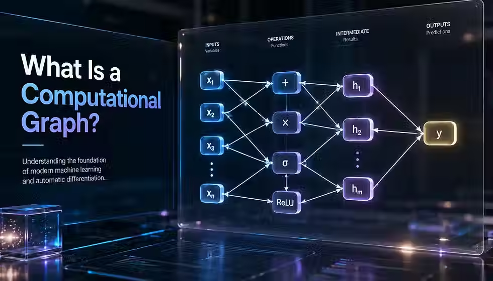
Every time a neural network learns something, thousands or millions of tiny arithmetic steps happen in a precise order, and then run in reverse. The structure that keeps that entire process organized, so a framework knows exactly what depends on what and exactly how to compute a gradient for every parameter, is called a computational graph. It sits quietly underneath almost every serious machine learning system in production today, from a fraud detector scoring a transaction in milliseconds to a large language model generating the next token, and understanding it turns TensorFlow, PyTorch, and JAX from black boxes into systems you can actually reason about.
TL;DR
A computational graph represents a computation as nodes (operations or values) connected by edges (data dependencies), most commonly forming a directed acyclic graph.
It exists so a framework can evaluate a computation in the correct order (the forward pass) and then apply the chain rule in reverse to compute gradients efficiently (the backward pass).
Automatic differentiation, not symbolic or numerical differentiation, is what frameworks use to compute those gradients, and backpropagation is reverse-mode automatic differentiation applied to a layered computation.
TensorFlow, PyTorch, and JAX all use graph-like representations internally, but they build, expose, and compile them differently: eager execution, tracing, and just-in-time compilation are not mutually exclusive.
Static versus dynamic graph construction is a useful teaching distinction, not a strict rule that still describes every modern framework accurately.
Graph representations unlock compiler-level optimizations, such as operator fusion and constant folding, that plain eager execution cannot access on its own.
What Is a Computational Graph?
A computational graph is a structured representation of a computation as a network of nodes and edges. Nodes represent operations or values (constants, variables, tensors), and edges represent the dependencies between them, showing which outputs feed into which operations. Machine learning frameworks evaluate these graphs to compute results and to calculate gradients through automatic differentiation.
Table of Contents
What Is a Computational Graph?
In plain English, a computational graph is a diagram-like structure that breaks a computation down into small, individual steps and records how those steps depend on one another. Instead of writing "y equals (a plus b) times c" as one opaque line, a computational graph stores it as separate operations, an addition and then a multiplication, connected by arrows that show which result feeds into which next step.
More technically, a computational graph is a data structure, typically a directed acyclic graph (DAG), in which nodes represent operations, values, or both, and directed edges represent data dependencies between them. Because the graph is directed and (in the common case) acyclic, there is always a valid order in which the operations can be executed so that every input is ready before the operation that needs it runs.
Computational graphs matter because they give a machine learning framework something a plain sequence of Python statements does not: an explicit, inspectable map of every dependency in a computation, which the framework can walk forward to compute a result and walk backward, using the chain rule, to compute every gradient it needs for training.
An Intuitive Mental Model
A useful way to picture a computational graph is as a recipe with intermediate steps, written out fully instead of compressed into one sentence. A recipe that says "whisk the eggs, fold them into the flour, then bake" already describes a small dependency graph: you cannot fold before whisking, and you cannot bake before folding. Each instruction is a node, and each "then" is an edge showing what has to happen first.
This analogy holds up well for explaining execution order and dependencies, but it starts to break down when you consider gradients. A recipe has no reverse pass; you cannot un-bake a cake to figure out how much the egg quantity influenced the final texture. A computational graph, by contrast, is built specifically so that this kind of reverse analysis, tracing an output's sensitivity back to every input, is possible and efficient. Keep the recipe analogy for intuition about structure and order, and set it aside once the discussion turns to gradients.
Anatomy of a Computational Graph
Different frameworks and diagrams use slightly different conventions, but most computational graphs are built from the following components.
Input nodes hold the data fed into the computation, such as a batch of images or a feature vector.
Constant nodes hold fixed values that do not change during execution, such as a hyperparameter or a literal number in an equation.
Variable nodes and trainable parameters hold values that the framework is allowed to update, most importantly the weights and biases of a model, sometimes discussed alongside model parameters and model weights.
Operation nodes represent a computation applied to one or more inputs, such as addition, matrix multiplication, or an activation function.
Intermediate values are the outputs of operation nodes that are not final results but are consumed by later operations.
Output nodes represent the final result of the graph, such as a prediction or a scalar loss value.
Directed edges connect nodes and represent dependencies: an edge from node A to node B means B needs A's result to run.
Tensor shapes and data types travel along the edges in most modern frameworks, since operations are usually defined for specific shapes and numeric types.
Leaf nodes are nodes with no incoming edges, typically inputs, constants, or parameters. Terminal or output nodes are nodes with no outgoing edges.
Topological ordering is the valid sequence in which nodes can be executed so every dependency is satisfied before it is needed; a directed acyclic graph always has at least one valid topological order.
Control dependencies are extra ordering constraints added for operations that have side effects, such as writing to a variable, where the natural data dependencies alone would not guarantee correct ordering.
Keep in mind that a hand-drawn diagram of a neural network's layers and the actual internal graph a framework builds are usually not the same object. A diagram might show one box labeled "Dense Layer," while the underlying execution graph expands that into several operations: a matrix multiplication, a bias addition, and an activation function applied element-wise. This distinction matters throughout the rest of this guide.
Turning an Equation into a Graph
The clearest way to understand a computational graph is to build one by hand. Consider this simple scalar expression:
y = (a + b) * c
Step 1: identify the operations. There are two elementary operations here: an addition and a multiplication. Introduce a name for the intermediate result of the addition, since the graph needs a node for it:
d = a + b
y = d * c
Step 2: identify the nodes. The graph has five nodes: three leaf nodes for the inputs (a, b, c), one intermediate node (d), and one output node (y).
Step 3: identify the edges. a and b both feed into the addition that produces d. d and c both feed into the multiplication that produces y.
Step 4: draw the graph. A simple text diagram of the dependency structure looks like this:
a ---\
      +--> [+] --> d ---\
 b ---/                  \
                          +--> [*] --> y
 c -----------------------/
Step 5: pick numeric values and evaluate. Let a = 2, b = 3, c = 4.
d = a + b = 2 + 3 = 5
y = d * c = 5 * 4 = 20
Step 6: forward evaluation order. The topological order is a, b, c (any order among the leaves), then d, then y. Nothing can be computed before its inputs exist, and the addition and multiplication cannot be reordered because the multiplication depends on d.
Step 7: local derivatives. Every operation node has a local derivative, the derivative of that single operation with respect to each of its own inputs, computed independently of everything else in the graph.
For d = a + b: the local derivative of d with respect to a is 1, and with respect to b is 1.
For y = d * c: the local derivative of y with respect to d is c, and with respect to c is d.
Step 8: the backward flow of gradients. The backward pass starts at the output with an upstream gradient of 1, since dy/dy = 1. It then multiplies upstream gradients by local derivatives, moving backward through the graph, which is exactly the chain rule applied mechanically, node by node.
dy/dd = (dy/dy) * (dy/dd) = 1 * c = 1 * 4 = 4
dy/dc = (dy/dy) * (dy/dc) = 1 * d = 1 * 5 = 5
dy/da = (dy/dd) * (dd/da) = 4 * 1 = 4
dy/db = (dy/dd) * (dd/db) = 4 * 1 = 4
Step 9: final derivatives. dy/da = 4, dy/db = 4, dy/dc = 5. You can verify this directly: y = (a + b) * c, so dy/da = c = 4, dy/db = c = 4, and dy/dc = (a + b) = 5. The graph-based reverse computation matches the direct algebraic derivative exactly, which is the entire point of automatic differentiation: it produces exact derivatives, not approximations.
Key idea: the backward pass never re-derives calculus rules at runtime. Each operation type, addition, multiplication, matrix multiplication, an activation function, ships with a small, fixed rule for how to turn an upstream gradient into gradients for its own inputs. The graph's job is to apply those local rules in the correct order and accumulate the results.
This scalar example scales directly to tensors. In a real model, a, b, and c become tensors (multi-dimensional arrays), the addition and multiplication become element-wise or matrix operations, and the same local-derivative-times-upstream-gradient pattern applies, just with tensors and Jacobians standing in for scalars and numbers. A dense neural network layer, z = Wx + b, is one more layer of the same pattern: a matrix multiplication node feeding into an addition node, both differentiable with the same local-derivative machinery.
The Forward Pass
The forward pass computes the graph's output by executing every node in a valid topological order, starting from the leaves (inputs, constants, parameters) and ending at the output (a prediction, or during training, a scalar loss). The graph's dependency structure is what determines this order; a node cannot execute until every node that feeds into it has already produced a value.
During training, most intermediate values computed in the forward pass need to be kept in memory, because the backward pass will need them to compute local derivatives. For example, the local derivative of y = d * c with respect to d is c, so the backward pass needs to know the value of c that was used during the forward pass. This is why training typically uses more memory than inference: inference only needs the forward pass, so a framework can discard intermediate activations as soon as they are no longer needed for the next forward step, since there will be no backward pass to consume them.
In a full training graph, the forward pass does not stop at the model's prediction. It continues through a loss function that compares the prediction to the true label and produces a single scalar loss value. That scalar is the starting point for the backward pass.
The Backward Pass and the Chain Rule
A derivative measures how much a function's output changes in response to a small change in one input. A gradient is the collection of derivatives of a scalar output (usually the loss) with respect to every input that matters, typically every trainable parameter in the model.
The backward pass computes gradients by applying the chain rule from calculus, which says that the derivative of a composed function is the product of the derivatives of its parts. In graph terms: for every node, the downstream gradient with respect to one of its inputs equals the upstream gradient (the gradient flowing in from the node that consumed this node's output) multiplied by the local derivative of this node with respect to that input.
Gradient accumulation happens when a single value feeds into more than one downstream operation. If a variable x is used in two separate places in the graph, its total gradient is the sum of the gradients flowing back along each path, not just one of them. This is a frequent source of subtle bugs when gradients are computed manually or when a framework's automatic accumulation is misunderstood.
A scalar loss is convenient specifically because reverse-mode differentiation is efficient when there is one output and many inputs: a single backward pass, starting from that one scalar, computes the gradient with respect to every parameter in the model in roughly the same amount of work as one forward pass. This is the property that makes training large models with millions or billions of parameters computationally feasible at all.
Why this matters: once the backward pass produces a gradient for every trainable parameter, an optimizer, such as stochastic gradient descent or Adam, uses those gradients to decide how to update each parameter. The optimizer step is related to the backward pass but is not the same computation: the backward pass answers "how sensitive is the loss to this parameter," while the optimizer answers "given that sensitivity, how should this parameter change." Conflating the two is one of the most common misunderstandings among newcomers to gradient descent-based training.
Automatic Differentiation Explained
There are four broad ways to obtain a derivative of a function implemented as code, and it helps to compare them directly.
Method | Mechanism | Accuracy | Cost | Advantages | Limitations | Typical use |
|---|---|---|---|---|---|---|
Manual differentiation | A person derives and codes the formula by hand | Exact, if done correctly | One-time human effort | Full control and insight | Slow, error-prone, does not scale to large models | Small, fixed formulas |
Numerical differentiation | Approximates f'(x) using finite differences, e.g. (f(x+h)-f(x))/h | Approximate; sensitive to round-off and truncation error | One or more extra forward evaluations per input dimension | Simple to implement, works on black-box functions | Inaccurate, scales poorly with many inputs | Gradient checking, debugging |
Symbolic differentiation | Manipulates an explicit mathematical expression to produce a new expression for the derivative | Exact | Can suffer from expression swell on complex programs | Produces a readable closed-form derivative | Struggles with control flow, loops, and large programs | Computer algebra systems |
Automatic differentiation | Applies the chain rule to elementary operations actually executed by the program, using recorded values, not symbolic expressions | Exact, up to floating-point precision | Roughly a small constant multiple of the forward pass cost in reverse mode | Exact, handles arbitrary code including control flow, scales to millions of parameters | Requires framework support; memory cost for storing intermediates | Neural network training, scientific computing |
Automatic differentiation (AD) is neither ordinary numerical differentiation nor purely symbolic differentiation, a distinction the foundational survey by Baydin, Pearlmutter, Radul, and Siskind makes explicit [10]. AD works by systematically applying the chain rule to the elementary operations a program actually performs, tracking numeric values (and their derivatives) as the program runs, rather than manipulating a symbolic formula or approximating with finite differences.
Forward-mode automatic differentiation propagates derivatives alongside values in the same direction as the original computation, computing how every intermediate value changes with respect to one chosen input at a time. It computes what is called a Jacobian-vector product. Forward mode tends to be advantageous when a function has relatively few input directions of interest and many outputs, because one forward-mode pass gives the derivative with respect to one input across all outputs at once.
Reverse-mode automatic differentiation runs the forward pass first, recording the operations performed, then propagates gradients backward from the output to every input in a single pass. It computes what is called a vector-Jacobian product. Reverse mode is advantageous when a function has many inputs and few outputs, such as a neural network with millions of parameters and one scalar loss, because a single backward pass produces gradients for every parameter at once [10].
Backpropagation, the algorithm most associated with neural network training, is a specialized and historically important application of reverse-mode automatic differentiation to layered computations. "Autodiff" and "backpropagation" are closely related but not perfect synonyms in every context: autodiff is the general technique, and backpropagation is what that technique looks like when applied to the specific structure of a feedforward or layered network.
Higher-order derivatives, such as a Hessian, are obtained by differentiating a derivative-computing function again; since the function that computes a gradient is itself just another program built from elementary operations, it can be differentiated with the same AD machinery, as demonstrated in JAX's ability to nest grad(grad(f)) directly [5].
Checkpointing, also called gradient recomputation, is a memory-saving trade-off in which a framework discards some intermediate activations during the forward pass and recomputes them during the backward pass instead of storing them, trading extra computation for lower peak memory use. This becomes important for very deep networks where storing every activation would exceed available memory.
Computational Graphs in Neural Networks
A small but complete neural network layer illustrates how a conceptual diagram expands into a real graph. Consider a single hidden layer with a softmax output, trained with cross-entropy loss:
z = W x + b
h = ReLU(z)
y_hat = softmax(U h + d)
L = cross_entropy(y_hat, y)
A layer diagram might draw this as two boxes: "Hidden Layer" and "Output Layer." The actual execution graph is more granular. The first line alone expands into a matrix multiplication node (Wx) and an addition node (+b), each with its own local derivative and its own entry in the backward pass. The ReLU activation is its own operation node, with a simple local derivative (1 where z is positive, 0 otherwise). The softmax function and the cross-entropy loss are each their own nodes, and in practice frameworks often fuse softmax and cross-entropy into a single combined operation for better numerical stability.
This is the sense in which a computational graph is a more general and more granular concept than a neural network architecture diagram. The architecture diagram communicates the model's design to a human reader; the computational graph is what the framework actually builds, evaluates, and differentiates. A single hidden layer in a diagram can correspond to a dozen or more nodes in the underlying graph once matrix multiplications, bias additions, and activation functions are broken out individually.
Static, Dynamic, Eager, Traced, and Compiled Execution
Machine learning frameworks differ in when they build a computational graph and how they turn Python code into something that can run efficiently on a GPU or TPU. It helps to define the terms precisely, since they are frequently used loosely.
Define-then-run (static) graph construction: the full graph is built first, as a distinct step, before any data flows through it. The graph can then be optimized once and executed many times.
Define-by-run (dynamic) graph construction: the graph is built incrementally, as operations actually execute, following the host language's normal control flow (loops, conditionals). This is how PyTorch's autograd behaves by default.
Eager execution: operations run immediately as they are called in Python, returning concrete results right away, with no separate graph-building step required for basic execution.
Tracing: a function is run once with placeholder or example inputs to record the sequence of operations it performs, producing a reusable graph-like representation without requiring the programmer to build the graph manually.
Ahead-of-time (AOT) compilation: a full program is compiled to an optimized, executable form before it ever runs on real data.
Just-in-time (JIT) compilation: compilation happens the first time a function is actually called with real (or representatively shaped) inputs, and the compiled version is reused on subsequent calls with compatible inputs.
Hybrid approaches: most modern frameworks combine several of these. Eager execution for development and debugging, tracing or JIT compilation for performance, and various forms of graph capture for deployment.
Approach | When graph/IR is created | Debugging experience | Optimization opportunity | Control-flow handling | Typical use case |
|---|---|---|---|---|---|
Define-then-run (classic static) | Before execution, as an explicit build step | Harder; errors surface when the graph runs, not when it's built | High; the whole graph is visible for optimization up front | Requires special graph-native control-flow ops | Deployment-heavy pipelines, older TF 1.x-style workflows |
Eager execution | No separate graph; each op runs immediately | Easiest; standard step-by-step debugging with normal tools | Low, unless later compiled | Native host-language control flow works directly | Prototyping, research, teaching |
Tracing (e.g. tf.function, jax.jit) | On first call, from a representative input | Moderate; retracing and Python side effects can surprise beginners | High for the traced path; poor for untraced branches | Data-dependent branches can be missed or require special handling | Production TensorFlow and JAX workloads |
Dynamic graph with JIT capture (e.g. PyTorch autograd + compilation) | Built per forward call; can additionally be captured/compiled | Close to eager; graph breaks can reduce optimization but preserve correctness | Medium to high, depending on how much of the graph compiles cleanly | Handles native Python control flow well in eager/dynamic mode | Research that still needs deployment performance |
Framework note: these categories are not mutually exclusive boxes. A single training script can use eager execution while prototyping, switch to a traced and compiled function for the performance-critical training loop, and export a further-optimized graph for deployment, all within the same framework and often the same codebase.
TensorFlow, PyTorch, and JAX
All three major frameworks build and use graph-like representations, but they differ meaningfully in workflow, defaults, and terminology.
TensorFlow
TensorFlow 2.x runs eagerly by default, executing operations immediately and returning concrete tensor values, which makes debugging straightforward [1]. The tf.function decorator transforms a Python function into one that is traced the first time it runs with a given input signature, producing a portable, graph-based representation (built on the underlying tf.Graph structure) that can be executed repeatedly without re-running the original Python code [2]. This traced graph is what enables SavedModel export for deployment, and it is also what TensorBoard's graph visualizer displays. Because tracing only captures the operations actually executed for a given input, TensorFlow requires some care with Python-level control flow and side effects; the guide's own advice is to write functions that operate on tensors rather than relying on external Python state [1][2]. Graph representations captured this way are also where Grappler-style and XLA-based graph optimizations are applied.
PyTorch
PyTorch normally runs in an eager, imperative style: operations execute immediately, and results are ordinary tensors you can inspect at any point. Underneath, PyTorch's autograd engine simultaneously builds a dynamic backward graph as the forward pass runs, and this graph is discovered anew on every call rather than being fixed in advance [3]. Every output tensor produced from an operation that requires gradients carries a grad_fn attribute, a reference to the function node that created it; following grad_fn references backward traces the graph back to the leaf tensors, the original inputs [4]. Setting requires_grad=True on a tensor tells autograd to track operations on it. Calling .backward() on a scalar output triggers the reverse traversal, populating the .grad attribute of each leaf tensor. detach() produces a new tensor that shares data but is disconnected from the graph, and the torch.no_grad() context manager disables graph construction entirely for code inside it, which is standard practice during inference. By default, the graph built for a backward pass is freed after that pass completes to save memory; passing retain_graph=True to backward() keeps it available for an additional backward call on the same graph. Modern PyTorch also offers graph capture and compilation tooling for performance, layered on top of this fundamentally dynamic, define-by-run foundation.
JAX
JAX takes a function-transformation approach built around pure functions. jax.grad takes a Python function and returns a new function that computes its gradient [5]. Under the hood, JAX transformations work by tracing: JAX runs the target function with abstract tracer objects standing in for real arrays, recording the sequence of primitive operations performed, without executing the underlying numerical work yet [8][9]. That recorded sequence is captured in JAX's own intermediate representation, the jaxpr (JAX expression), an explicitly typed, functional, first-order representation of the program in algebraic normal form [7]. jax.jit uses this same tracing mechanism to compile a function ahead of repeated calls, handing the resulting representation to the XLA compiler for hardware-specific optimization [9]. Because JAX's transformations compose, jit, grad, and vmap (automatic vectorization) can be stacked freely, and because tracing assumes the traced function is pure, JAX expects functions without hidden side effects or in-place mutation of external state for transformations to behave predictably.
None of these frameworks is simply "static" or "dynamic" anymore; each combines eager execution, tracing, and compilation in different proportions and with different defaults, and the details of exactly how much of a given program compiles cleanly can change between framework versions, so specific performance or coverage claims are always worth checking against current documentation rather than assumed from general reputation.
Code Examples
The following examples are minimal and intended to demonstrate the concepts above, not to be a complete tutorial. The scalar example matches the worked example earlier in this guide, so the numbers can be checked directly.
A framework-independent scalar example
This plain Python version implements the forward and backward pass manually, exactly as derived earlier, with no machine learning library involved.
# Forward pass: y = (a + b) * c
a, b, c = 2.0, 3.0, 4.0
d = a + b        # d = 5.0
y = d * c        # y = 20.0

# Backward pass, starting from dy/dy = 1
dy_dy = 1.0
dy_dd = dy_dy * c   # local derivative of (d*c) w.r.t. d is c -> 4.0
dy_dc = dy_dy * d   # local derivative of (d*c) w.r.t. c is d -> 5.0
dy_da = dy_dd * 1.0 # local derivative of (a+b) w.r.t. a is 1 -> 4.0
dy_db = dy_dd * 1.0 # local derivative of (a+b) w.r.t. b is 1 -> 4.0

print(y, dy_da, dy_db, dy_dc)
# Expected output: 20.0 4.0 4.0 5.0
PyTorch autograd
PyTorch tracks the same computation automatically once requires_grad is enabled, and .backward() performs the reverse pass.
import torch

a = torch.tensor(2.0, requires_grad=True)
b = torch.tensor(3.0, requires_grad=True)
c = torch.tensor(4.0, requires_grad=True)

d = a + b
y = d * c
y.backward()

print(y.item(), a.grad.item(), b.grad.item(), c.grad.item())
# Expected output: 20.0 4.0 4.0 5.0
TensorFlow gradient with GradientTape
TensorFlow records operations for differentiation inside a GradientTape context, then computes gradients with respect to the watched tensors.
import tensorflow as tf

a = tf.Variable(2.0)
b = tf.Variable(3.0)
c = tf.Variable(4.0)

with tf.GradientTape() as tape:
    d = a + b
    y = d * c

grads = tape.gradient(y, [a, b, c])
print(y.numpy(), [g.numpy() for g in grads])
# Expected output: 20.0 [4.0, 4.0, 5.0]
JAX grad
JAX differentiates a pure function directly; jax.grad returns a new function that computes the gradient with respect to the chosen argument.
import jax
import jax.numpy as jnp

def f(a, b, c):
    d = a + b
    y = d * c
    return y

grad_f = jax.grad(f, argnums=(0, 1, 2))
grads = grad_f(2.0, 3.0, 4.0)
print(f(2.0, 3.0, 4.0), grads)
# Expected output: 20.0 (4.0, 4.0, 5.0)
All four examples agree on the same result derived by hand earlier: y = 20 and gradients of 4, 4, and 5 with respect to a, b, and c. That agreement is the practical proof that automatic differentiation, however a given framework implements it internally, is computing exact derivatives from the same underlying chain-rule logic.
Graph Optimization
Once a computation exists as an explicit graph, whether through tracing, explicit graph-building, or ahead-of-time compilation, a compiler can analyze and rewrite it before execution in ways that are difficult or impossible to do safely on code that is only ever interpreted one operation at a time. Common optimizations include:
Constant folding, computing parts of the graph that depend only on constants at compile time instead of on every run [11].
Dead-code elimination, removing nodes whose outputs are never used by anything downstream.
Common-subexpression elimination, merging duplicate computations that produce identical results, evaluating them once instead of repeatedly [11].
Operator fusion, combining multiple operations into a single kernel to avoid writing and re-reading intermediate results to memory between each step, a major source of speedup on GPUs and TPUs [12][13].
Algebraic simplification, rewriting mathematically equivalent but cheaper expressions, such as replacing multiplication by one or zero with a no-op.
Kernel selection, choosing the fastest available low-level implementation of an operation for the specific hardware in use.
Parallel scheduling and device placement, deciding which operations can run concurrently and which physical device (CPU, GPU, TPU) should execute each one.
Memory planning and buffer reuse, deciding when intermediate buffers can be freed and reused rather than allocated fresh for every step.
Communication optimization, reducing the volume and frequency of data transferred between devices in distributed or multi-accelerator training.
XLA (Accelerated Linear Algebra), used by both TensorFlow and JAX, performs several of these passes on a graph-level intermediate representation before handing the result to hardware-specific backends for further, target-specific optimization [11]. The exact set of optimizations that applies to a given program depends heavily on the framework, the compiler version, the target hardware, and the specific structure of the computation, so treat any single optimization as a general tendency rather than a guaranteed transformation for every graph.
Benefits of Computational Graphs
Automatic gradient computation through reverse-mode automatic differentiation, without hand-deriving calculus for every new model architecture.
Efficient execution, since the framework can schedule, batch, and optimize operations instead of executing naive, unoptimized Python line by line.
Parallelism, because independent branches of the graph, wherever the dependency structure allows it, can run concurrently.
Hardware acceleration, since a graph representation can be lowered to GPU, TPU, or other accelerator-specific code.
Portability, since a saved graph can often run in environments without the original Python code, such as mobile or embedded deployment.
Serialization and deployment, since a graph can be saved, versioned, and loaded independently of the training script that produced it.
Visualization, since a graph's explicit structure can be rendered visually for inspection, as with TensorBoard's graph viewer.
Debugging and optimization tooling, since profilers and debuggers can attach to well-defined graph nodes.
Distributed execution, since a graph's dependency structure tells a distributed runtime which operations can be split across machines and which must stay synchronized.
A reproducible representation of a computation, useful for auditing, comparing model versions, or reasoning about a system independently of the code that generated it.
Not every graph system provides every one of these benefits automatically; the degree of parallelism, portability, or optimization actually achieved depends on the framework, the target hardware, and how the graph was constructed.
Limitations and Trade-Offs
Memory consumption from storing activations needed for the backward pass, which can dominate total memory use for deep networks.
Graph-construction or tracing overhead, since building or tracing a graph is not free, particularly the first time a function runs.
Retracing, which happens when a traced function is called with a new input shape or type, forcing the framework to rebuild its internal representation.
Shape specialization, since compiled graphs are often specialized to particular tensor shapes and may need to recompile for new ones.
Data-dependent control flow, where the path taken through a computation depends on runtime values, which some tracing and compilation systems handle awkwardly or not at all.
Side effects and mutability, since in-place operations and external state can conflict with a framework's assumptions about pure or replayable computations.
Unsupported operations, since a given compiler backend may not support every operation a framework's eager mode allows.
Debugging compiled graphs, which is generally harder than debugging eager code, since compiled execution can obscure the mapping between a runtime error and a specific line of Python.
Graph breaks, points where a compiler falls back to eager execution because it cannot trace through a piece of code, which can silently reduce optimization without producing an error.
Compilation latency, the delay incurred the first time a function is traced or compiled, which matters for workloads with many distinct input shapes.
Numerical instability, and the related problems of vanishing and exploding gradients, which are properties of the underlying math and architecture rather than of the graph representation itself, but which are diagnosed and addressed by inspecting how gradients flow through the graph.
Common Mistakes and Debugging Issues
Most gradient-related bugs trace back to a small set of recurring mistakes, though the exact symptoms and framework-specific error messages vary.
Accidentally detaching a tensor (for example with detach() in PyTorch) and then being surprised that no gradient flows through it.
Disabling gradient tracking unintentionally, such as leaving code inside a no_grad() or stop_gradient context that was meant only for a small part of the computation.
Updating values in place in a way that corrupts values the backward pass still needs, which frameworks often detect and raise an error for, but not always immediately.
Expecting gradients on non-leaf tensors, when by default only leaf tensors accumulate a .grad attribute after backward().
Forgetting to clear accumulated gradients between training steps, since gradients accumulate by addition rather than being reset automatically in some workflows.
Calling backward multiple times after a graph has already been released, since by default the backward graph is freed after one use unless retain_graph is set.
Building a new graph on every unintended iteration, for example inside a loop that should have been vectorized, which wastes memory and time re-tracing or reconstructing structure that never changes.
Triggering repeated tracing or compilation by calling a traced function with constantly changing input shapes or Python-level arguments.
Breaking the graph by converting a tensor to a plain host-language value (for example calling .item() or float() too early), which severs the connection autograd needs to track that value.
Mismatched shapes, a frequent and usually loud error, but sometimes silent when broadcasting rules apply in an unintended way.
Assuming every operation is differentiable, when some operations (indexing with certain conditions, non-differentiable functions like argmax) do not have a meaningful gradient and will either error or silently produce a zero or undefined gradient.
Confusing a zero gradient with a missing gradient, since a gradient of exactly zero for a legitimate reason looks identical, at first glance, to a bug that prevented the gradient from being computed at all.
Computational Graph Misconceptions
"A computational graph is the same thing as a neural network." A neural network can be represented as a computational graph, but the graph concept is more general and applies far beyond neural networks, including to scientific computing and differentiable simulation.
"Every computational graph is static." Dynamic, define-by-run graphs, as used by PyTorch's autograd by default, are built fresh on every forward pass and are just as much a computational graph as any pre-built static graph.
"Dynamic graphs cannot be optimized." Modern frameworks apply graph capture, tracing, and compilation on top of dynamically constructed computations to recover many of the optimization benefits historically associated only with static graphs.
"Backpropagation and gradient descent are the same process." Backpropagation computes gradients; gradient descent (or a variant like Adam) uses those gradients to update parameters. They are distinct, sequential steps in a training loop.
"Automatic differentiation is symbolic differentiation." AD works on the actual sequence of numeric operations a program executes, not on a symbolic mathematical expression, which is why it handles arbitrary code, including loops and conditionals, that symbolic differentiation struggles with.
"The graph stores only operations." Graphs also encode values, shapes, data types, and, in many implementations, control dependencies needed for correct execution order around side effects.
"Edges always mean exactly the same thing in every diagram." Depending on the convention, an edge might represent a tensor, a data dependency, a control dependency, or simply an ordering constraint; always check what a given diagram's edges are meant to convey.
"A graph must be manually created by the programmer." Most modern usage builds the graph automatically, either by tracing eager Python code or by recording operations as they execute, without the programmer explicitly constructing nodes and edges.
"Computational graphs are useful only during training." Graphs are also central to inference optimization, deployment, serialization, and scientific and engineering applications that never involve gradient-based training at all.
"A framework's visible Python code is always identical to its compiled internal graph." Tracing and compilation can fuse, reorder, eliminate, or specialize operations, so the compiled graph frequently differs structurally from a literal reading of the source code, while still computing the same result.
Related Concepts and Distinctions
Graph data structure (general computer science): the general-purpose data structure of nodes and edges; a computational graph is one specific application of it, where edges also encode a computational meaning.
Graph neural network: a neural network architecture that operates on graph-structured input data (like a social network or molecule); this is a completely different use of the word "graph" from the internal execution graph a framework builds to run and differentiate any model, including a graph neural network itself.
Neural network architecture diagram: a human-facing illustration of a model's layers, typically far less granular than the operation-level computational graph the framework actually executes.
Dataflow graph: a general model of computation where nodes are operations and edges represent data moving between them; a computational graph is essentially a dataflow graph specialized for numerical computation and differentiation.
Dependency graph: any graph showing what depends on what (common in build systems and package managers); a computational graph is a dependency graph whose nodes happen to be numerical operations.
Abstract syntax tree (AST): a tree representation of source code's grammatical structure, produced by a compiler's parser; a computational graph instead represents the semantics and data dependencies of a numeric computation, often built from or alongside an AST but conceptually distinct from it.
Execution plan: a scheduling and resource-assignment plan for running a set of operations (common in databases and distributed systems); a computational graph can be an input to an execution plan, but the plan also includes decisions like device placement and timing.
Intermediate representation (IR): any program representation a compiler uses between source code and final output; a jaxpr or an XLA HLO graph are specific examples of an IR used for numerical computation.
Computation tree: a tree-shaped special case where every value is used exactly once; most real computational graphs are not trees, because values like shared weights are frequently reused by multiple downstream operations.
Bayesian network: a directed acyclic graph representing probabilistic dependencies between random variables, used for probabilistic reasoning rather than for evaluating or differentiating a deterministic numeric computation.
Real-World Applications
Computational graphs are not confined to a single use case; they show up anywhere a system needs to evaluate a complex numeric computation and, often, differentiate it.
Deep learning training, where the graph structures both the forward prediction and the backward gradient computation for every parameter update.
Inference deployment, where a trained, often further-optimized graph is exported and served in production, sometimes on very different hardware from where it was trained.
Scientific computing, where large systems of equations are broken into dependency graphs for numerical solvers.
Differentiable simulation, where physical simulations are built from differentiable operations so gradients can flow through an entire simulated process, useful in physics-informed neural networks.
Robotics, where differentiable models of dynamics and control support planning and learning-based control.
Computer vision, where convolutional and vision transformer architectures are themselves large computational graphs trained end to end.
Natural language processing, where transformer models and their attention mechanisms are expressed and differentiated as computational graphs.
Reinforcement learning, where policy and value networks are trained through gradients computed over graphs that may also include the differentiable parts of an environment model.
Probabilistic programming, where graphs represent dependencies among random variables and support both inference and gradient-based optimization of model parameters.
General optimization problems, wherever gradients of a numeric objective with respect to many variables are needed efficiently.
Physics-informed machine learning, where a model's loss includes terms derived from physical equations, differentiated through the same graph as the rest of the network.
Compiler systems for numerical programs, where the graph itself is the object being analyzed, optimized, and lowered to hardware-specific code, as in XLA and MLIR-based toolchains.
A Short History
Ideas underlying automatic differentiation trace back to the 1950s and 1960s, well before their prominent use in machine learning [10]. Dataflow-graph thinking, representing a program as nodes and data-dependency edges, developed separately in computer science as a general model of parallel and distributed computation. Backpropagation, the specific reverse-mode differentiation procedure now central to neural network training, was independently derived multiple times before becoming widely known in the machine learning community in the 1980s. Early deep learning libraries in the 2000s and early 2010s largely used explicit, define-then-run static graphs, since building the graph once and executing it many times suited the hardware and tooling constraints of the time.
Later frameworks introduced define-by-run systems, building the graph dynamically as Python code executed, which improved debuggability and made research iteration faster at some initial cost to deployment performance. The current generation of major frameworks has largely converged on hybrid designs: eager, imperative execution as the default developer experience, combined with tracing, graph capture, and just-in-time compilation layered on top for performance and deployment, so that the historical "static versus dynamic" split is now better understood as a spectrum of techniques a single framework can use in different parts of the same program.
How Deep Do You Need to Understand This?
A beginner training standard models mainly needs the intuition from the worked example: forward pass computes a result, backward pass computes gradients, and an optimizer uses those gradients to update parameters.
A practitioner debugging gradients needs the material on common mistakes and misconceptions: detached tensors, disabled gradient tracking, and accumulation bugs account for the large majority of real-world gradient problems.
A researcher creating custom differentiable operations needs a working understanding of local derivatives, upstream and downstream gradients, and how a given framework expects custom gradient rules to be registered.
A compiler or framework engineer needs the material on graph optimization, tracing, jaxpr-style intermediate representations, and how XLA-style compilers transform a graph before it reaches hardware.
A production engineer optimizing deployment needs to understand graph capture, shape specialization, retracing, and the trade-offs between eager flexibility and compiled performance discussed in the execution-modes section above.
FAQ
Is a computational graph the same as a neural network?
No. A neural network can be represented as a computational graph, but the graph concept is more general. Computational graphs also appear in scientific computing, robotics, and any other domain that needs to evaluate and often differentiate a numeric computation, with or without a neural network involved.
Do I need to build a computational graph by hand?
Almost never in modern practice. TensorFlow, PyTorch, and JAX all build the relevant graph or trace automatically, either as you write ordinary tensor operations (PyTorch autograd, TensorFlow eager mode) or when you apply a transformation like tf.function or jax.jit to a function.
What is the difference between the forward pass and the backward pass?
The forward pass evaluates the graph to produce an output, such as a prediction or a loss value, executing nodes in dependency order. The backward pass starts from that output and applies the chain rule in reverse to compute the gradient of the output with respect to every input or parameter that needs one.
Is automatic differentiation the same as symbolic differentiation?
No. Symbolic differentiation manipulates an explicit mathematical expression to produce a new expression for the derivative, and can suffer from expression swell on complex programs. Automatic differentiation instead applies the chain rule to the actual sequence of elementary operations a program executes, tracking numeric values as it goes, which lets it handle arbitrary code, including loops and conditionals.
Is backpropagation the same thing as automatic differentiation?
Backpropagation is a specific, well-known application of reverse-mode automatic differentiation to layered computations like neural networks. Automatic differentiation is the more general technique; backpropagation is one important instance of it, not a separate technique.
Why does reverse mode work so well for training neural networks?
Because a training objective is a single scalar loss and the model can have millions of parameters. Reverse-mode automatic differentiation computes the gradient with respect to every parameter in roughly one backward pass, regardless of how many parameters there are, which is dramatically cheaper than computing each parameter's derivative separately.
Is TensorFlow always static and PyTorch always dynamic?
No, and this common description is outdated. TensorFlow 2.x runs eagerly by default and only builds a graph when tf.function traces a function. PyTorch builds a dynamic graph by default through autograd but also offers graph capture and compilation tooling for performance. Both frameworks combine eager execution with graph-based compilation in different proportions.
What is a jaxpr?
A jaxpr, short for JAX expression, is JAX's internal intermediate representation of a traced program: an explicitly typed, functional, first-order representation in algebraic normal form. JAX transformations like jax.jit and jax.grad work by tracing a Python function into a jaxpr and then interpreting or compiling that representation.
Why do I sometimes get 'None' when I check a tensor's gradient in PyTorch?
The most common reasons are that the tensor is not a leaf tensor (only leaf tensors accumulate .grad by default), that requires_grad was never set to True, that the tensor was detached from the graph, or that the computation happened inside a no_grad() context.
What is the difference between a graph break and a normal error?
A graph break happens when a compiler cannot trace or compile a piece of code and falls back to running it eagerly instead of raising an error. The program still produces a correct result, but it may run slower than expected because part of the computation missed out on compiled optimizations.
Can computational graphs have loops or cycles?
The dependency structure that a single forward-and-backward pass evaluates is acyclic; a node cannot depend on its own not-yet-computed output. Iterative processes like recurrent computations or training loops are handled by repeating or unrolling the acyclic structure over time steps, or through special control-flow constructs, rather than by putting an actual cycle in the graph.
Does inference use a computational graph too?
Yes. Inference still evaluates the forward pass of the graph to produce a prediction. It simply skips the backward pass, and frameworks often free intermediate values immediately after use during inference since there is no gradient computation that will need them later.
What is checkpointing in the context of computational graphs?
Checkpointing, or gradient recomputation, is a memory-saving technique where some intermediate activations are deliberately not stored during the forward pass and are recomputed during the backward pass instead. It trades additional computation for reduced peak memory usage, which matters most for very deep or very large models.
Why does my traced function recompile every time I call it?
Tracing-based systems like tf.function and jax.jit typically specialize the compiled graph to the shapes, dtypes, and sometimes Python-level values of the inputs seen during tracing. Calling the function with a new input shape, dtype, or a changed static argument triggers retracing and recompilation, which can be a significant, avoidable source of slowdown.
Key Takeaways
A computational graph breaks a computation into nodes (operations or values) and edges (dependencies), almost always forming a directed acyclic graph for any single forward-and-backward evaluation.
The forward pass evaluates the graph in dependency order; the backward pass applies the chain rule in reverse to compute exact gradients.
Automatic differentiation is distinct from both numerical and symbolic differentiation; it works on the actual sequence of operations a program executes.
Reverse-mode automatic differentiation, the basis of backpropagation, is efficient precisely when there are many inputs (parameters) and one scalar output (loss).
Static versus dynamic graph construction is a spectrum, not a strict binary; TensorFlow, PyTorch, and JAX each blend eager execution, tracing, and compilation.
A layer diagram and the actual operation-level execution graph are usually not the same object; the graph is more granular.
Graph-level optimizations like operator fusion, constant folding, and common-subexpression elimination require an explicit graph representation to apply.
Most gradient bugs, detached tensors, disabled tracking, unintended accumulation, trace back to a small, well-known set of common mistakes.
Actionable Next Steps
Draw the graph for y = (a + b) * c on paper, then extend it to a second operation of your choosing, and verify your backward pass by hand against the direct algebraic derivative.
Pick one framework (PyTorch, TensorFlow, or JAX) and run the corresponding code example from this guide, then modify the input values and confirm the printed gradients still match your own hand calculation.
In PyTorch, print a tensor's .grad_fn after a few chained operations and trace the printed function names back to the operations you wrote.
In TensorFlow, wrap a small function with tf.function, call it with two different input shapes, and observe when retracing happens.
In JAX, call jax.make_jaxpr on a small function to see its traced intermediate representation directly.
Deliberately introduce one of the common mistakes described above, such as calling .detach() before .backward(), and observe exactly how the framework responds.
Read the official tf.function, PyTorch autograd, and JAX automatic differentiation guides linked in the Sources & References section below, since framework details evolve and official documentation stays current in a way a single article cannot.
Glossary
Automatic differentiation (AD): A family of techniques for computing exact derivatives of a function implemented as code, by applying the chain rule to the elementary operations the program actually performs.
Backpropagation: A specific, widely used application of reverse-mode automatic differentiation to layered computations such as neural networks.
Chain rule: The calculus rule stating that the derivative of a composed function equals the product of the derivatives of its parts, applied node by node during the backward pass.
Checkpointing: A memory-saving technique that recomputes some intermediate values during the backward pass instead of storing them from the forward pass.
Computational graph: A structured representation of a computation as nodes (operations or values) connected by edges (data dependencies).
Constant folding: A graph optimization that precomputes parts of a graph depending only on constants at compile time.
Directed acyclic graph (DAG): A graph whose edges have direction and which contains no cycles, guaranteeing a valid execution order exists.
Downstream gradient: The gradient computed for one of a node's inputs, derived from the upstream gradient multiplied by the local derivative.
Eager execution: An execution mode where operations run immediately and return concrete results, without a separate graph-building step.
Forward pass: The evaluation of a computational graph from inputs to outputs, in dependency order.
Forward-mode automatic differentiation: A form of automatic differentiation that propagates derivatives in the same direction as the original computation, efficient for functions with few inputs and many outputs.
Gradient: The collection of derivatives of a scalar output with respect to every input or parameter of interest.
Gradient accumulation: The summing of gradients that flow back to a value along more than one path in the graph.
Grad_fn: In PyTorch, an attribute on a tensor referencing the function that produced it, used to build the backward graph.
Jaxpr: JAX's internal, explicitly typed, functional intermediate representation of a traced program.
Leaf tensor: A tensor at the edge of the computation graph, typically an original input, with no operation that produced it inside the tracked graph.
Local derivative: The derivative of a single operation with respect to one of its own inputs, computed independently of the rest of the graph.
Node: An element of a computational graph representing an operation, a value, or both.
Operator fusion: A graph optimization combining multiple operations into a single kernel to reduce memory traffic and launch overhead.
Reverse-mode automatic differentiation: A form of automatic differentiation that computes gradients by traversing the graph backward from output to inputs, efficient for functions with many inputs and one (or few) outputs.
Retracing: The process of rebuilding a traced function's internal representation when it is called with a new, incompatible input signature.
Tensor: A multi-dimensional array, the basic data structure operations in a computational graph typically consume and produce.
Topological order: A valid ordering of a graph's nodes in which every node appears after all the nodes it depends on.
Tracing: Running a function once with representative inputs to record the sequence of operations it performs, producing a reusable graph-like representation.
Upstream gradient: The gradient flowing into a node from whatever consumed its output, used together with the local derivative to compute downstream gradients.
Vector-Jacobian product (VJP): The core operation performed at each step of reverse-mode automatic differentiation.
XLA (Accelerated Linear Algebra): A domain-specific compiler used by TensorFlow and JAX to optimize and compile graph-level computations for specific hardware.
Sources & References
[1] Google. "Introduction to graphs and tf.function." TensorFlow Core Guide. Accessed July 26, 2026. https://www.tensorflow.org/guide/intro_to_graphs
[2] Google. "Better performance with tf.function." TensorFlow Core Guide. Accessed July 26, 2026. https://www.tensorflow.org/guide/function
[3] PyTorch. "Autograd mechanics." PyTorch Documentation. Accessed July 26, 2026. https://docs.pytorch.org/docs/stable/notes/autograd.html
[4] PyTorch. "The Fundamentals of Autograd." PyTorch Tutorials. Accessed July 26, 2026. https://docs.pytorch.org/tutorials/beginner/introyt/autogradyt_tutorial.html
[5] Google / JAX Authors. "Automatic differentiation." JAX Documentation. Accessed July 26, 2026. https://docs.jax.dev/en/latest/automatic-differentiation.html
[6] Google / JAX Authors. "The Autodiff Cookbook." JAX Documentation. Accessed July 26, 2026. https://docs.jax.dev/en/latest/notebooks/autodiff_cookbook.html
[7] Google / JAX Authors. "JAX internals: The jaxpr language." JAX Documentation. Accessed July 26, 2026. https://docs.jax.dev/en/latest/jaxpr.html
[8] Google / JAX Authors. "Key concepts." JAX Documentation. Accessed July 26, 2026. https://docs.jax.dev/en/latest/key-concepts.html
[9] Google / JAX Authors. "Tracing." JAX Documentation. Accessed July 26, 2026. https://docs.jax.dev/en/latest/tracing.html
[10] Baydin, A. G., Pearlmutter, B. A., Radul, A. A., & Siskind, J. M. "Automatic Differentiation in Machine Learning: a Survey." Journal of Machine Learning Research, 18, 2018 (first published 2015). https://www.jmlr.org/papers/volume18/17-468/17-468.pdf
[11] OpenXLA Project. "XLA architecture." OpenXLA Documentation, GitHub. Accessed July 26, 2026. https://github.com/openxla/xla/blob/main/docs/architecture.md
[12] Snider, D., & Liang, R. "Operator Fusion in XLA: Analysis and Evaluation." arXiv preprint, 2023. https://arxiv.org/pdf/2301.13062
[13] PyTorch. "PyTorch/XLA Overview." PyTorch/XLA Documentation. Accessed July 26, 2026. https://docs.pytorch.org/xla/master/learn/xla-overview.html
[14] Google. "Introduction to gradients and automatic differentiation." TensorFlow Core Guide. Accessed July 26, 2026. https://www.tensorflow.org/guide/autodiff


